Mode Locking

A continuous-wave laser concentrates energy into a narrow optical-frequency region. A mode-locked laser instead organizes many longitudinal modes into a phase-coherent superposition whose intensity is concentrated into a periodic train of short pulses. The central physics is interference:

$$\text{broad coherent spectrum} + \text{stable relative spectral phase} \longrightarrow \text{short reproducible waveform}.$$

Mode locking is not merely the simultaneous oscillation of many modes. Nor does it require every modal phase to be numerically equal. It requires the relative phases to obey a stable relation from one round trip to the next. A constant phase changes the carrier phase, a phase linear in frequency shifts the pulse in time, and nonlinear spectral phase broadens or reshapes the pulse.

Canonical Scope

This page owns:

1. the frequency-domain meaning of phase locking among longitudinal modes;
2. the derivation of a periodic pulse train from an equally spaced mode set;
3. active amplitude and phase modulation;
4. passive saturable-absorber, Kerr-lens, and nonlinear-polarization mechanisms;
5. the semiclassical master-equation view of a stable circulating pulse;
6. transform-limited Gaussian and $\operatorname{sech}^2$ bandwidth–duration products;
7. chirp and group-delay-dispersion broadening;
8. pulse-energy, peak-power, autocorrelation, FROG, and SPIDER conventions;
9. common mode-locking instabilities and their diagnosis;
10. the connection to time resolution in ultrafast spectroscopy.

Optical Cavities owns free spectral range, finesse, linewidth, photon lifetime, and cavity stability. Laser Modes owns longitudinal and transverse eigenmodes. Gain and Threshold owns round-trip gain and mode competition. Linewidth and Coherence owns continuous-wave optical phase and frequency noise. Ultrafast Spectroscopy Overview owns pump–probe observables and material dynamics. Frequency Combs owns comb-tooth frequencies, carrier-envelope offset self-referencing, optical division, and frequency metrology.

Two Times and Three Frequencies

Mode-locked laser notation mixes several scales, so declare them first.

• $\tau$ is fast time within one round-trip window.
• $T$ is slow time, measuring evolution over many round trips.
• $T_{\rm rt}$ is the cavity round-trip time.
• $f_{\rm rep}=1/T_{\rm rt}$ is the fundamental pulse repetition frequency.
• $\Omega_{\rm FSR}=2\pi f_{\rm rep}$ is the angular free spectral range.
• $\omega_0$ is an optical carrier angular frequency.
• $\Omega=\omega-\omega_0$ is an angular-frequency offset from the carrier.

For a linear cavity of optical length $L_{\rm opt}$, $T_{\rm rt}=2L_{\rm opt}/c$; for a ring cavity, $T_{\rm rt}$ is the single-loop group delay. Dispersion makes the mode spacing weakly frequency-dependent, so the constant-spacing formulas below are local approximations around $\omega_0$.

The positive-frequency field is written

$$\mathcal E^{(+)}(t) = \frac{1}{2} A(t)e^{-i\omega_0t}.$$

The slowly varying envelope $A$ contains the pulse shape and phase. Factors of $1/2$ depend on field convention and do not affect the normalized interference results.

Frequency Modes and Phases

Longitudinal comb before locking

Over a bandwidth small enough that the free spectral range is nearly constant, the cavity resonances can be indexed as

$$\omega_q \simeq \omega_{\rm c} + q\Omega_{\rm FSR}, \qquad q\in\mathbb Z.$$

If several resonances oscillate, write

$$\mathcal E^{(+)}(t) = \frac{1}{2} \sum_q a_q e^{i\phi_q} e^{-i\omega_qt}.$$

The power spectrum gives $|a_q|^2$, but not the phases $\phi_q$. Equal line spacing alone therefore does not imply pulses. If the phases wander independently, modal beating produces an irregular intensity pattern. A stable pulse train requires a reproducible spectral phase function $\phi(\omega_q)$.

What “locked” means

The simplest locked relation is affine in mode index,

$$\phi_q = \phi_{\rm c} + q\phi_{\rm s}.$$

Substitution gives

$$\begin{aligned} \mathcal E^{(+)}(t) &= \frac{1}{2} e^{i\phi_{\rm c}} e^{-i\omega_{\rm c}t} \sum_q a_q e^{-iq(\Omega_{\rm FSR}t-\phi_{\rm s})}. \end{aligned}$$

The constant $\phi_{\rm c}$ changes an overall optical phase. The slope $\phi_{\rm s}$ shifts the envelope by

$$t_0 = \frac{\phi_{\rm s}}{\Omega_{\rm FSR}}.$$

Thus all phases equal is only one choice of time origin. The invariant statement is that phase differences are fixed. More generally,

$$\phi_q = \phi_{\rm c} + q\phi_{\rm s} + \delta\phi_q,$$

where a stable but nonlinear residual $\delta\phi_q$ produces a reproducible chirped or structured pulse. Random or time-dependent residuals reduce the coherent peak and generate timing, phase, or shape noise.

Adjacent-mode coupling

A modulation or nonlinearity at the mode spacing couples neighboring cavity modes. In a frequency-domain coupled-mode picture,

$$\frac{d a_q}{dT} \supset \mu_+ a_{q-1} + \mu_- a_{q+1}.$$

The coupling coefficients carry the modulation phase and can make a particular phase relation dynamically preferred. In the time domain, the same operation is a periodic loss, gain, or phase gate. Frequency-domain mode coupling and time-domain pulse shaping are Fourier-dual descriptions of one process.

Pulse-Train Formation

Finite equal-amplitude mode set

Take $M=2N+1$ modes with equal amplitude $A_0$, equal phase at $t=0$, and spacing $\Omega_{\rm FSR}$. Their envelope is

$$\begin{aligned} A(t) &= A_0 \sum_{m=-N}^{N} e^{-im\Omega_{\rm FSR}t} \\ &= A_0 \frac{ \sin\!\left(M\Omega_{\rm FSR}t/2\right) }{ \sin\!\left(\Omega_{\rm FSR}t/2\right) }. \end{aligned}$$

The ratio is a Dirichlet kernel. At

$$t = \ell T_{\rm rt}, \qquad T_{\rm rt} = \frac{2\pi}{\Omega_{\rm FSR}}, \qquad \ell\in\mathbb Z,$$

all $M$ phasors add in phase. The limiting field amplitude is $MA_0$, so the peak intensity scales as $M^2|A_0|^2$. Away from those times, destructive interference suppresses the field.

The time-averaged intensity is proportional to

$$\left\langle |A(t)|^2\right\rangle = \sum_{m=-N}^{N}|A_0|^2 = M|A_0|^2,$$

because cross terms average to zero over one round trip. Concentrating the same average power into a fraction of the period therefore raises the peak power by a factor of order $M$.

The central lobe has a width of order

$$\Delta t \sim \frac{T_{\rm rt}}{M} \sim \frac{1}{M f_{\rm rep}},$$

consistent with the total coherent bandwidth $\Delta\nu\sim M f_{\rm rep}$. Exact numerical widths depend on the spectral amplitude envelope and on the chosen FWHM or rms convention.

Arbitrary spectral envelope

Let the complex spectral amplitudes be samples of a smooth envelope $\widetilde A(\Omega)$ at $\Omega_q=q\Omega_{\rm FSR}$. The periodic time-domain envelope is

$$A_{\rm per}(t) = \sum_q \widetilde A(q\Omega_{\rm FSR}) e^{-iq\Omega_{\rm FSR}t}.$$

Up to Fourier-normalization factors, this is a periodic replication of the inverse transform of $\widetilde A(\Omega)$. The longitudinal-mode spacing sets the pulse period, while the occupied coherent bandwidth and spectral phase set the waveform inside each period.

This separates two often-confused statements:

$$\begin{aligned} \text{mode spacing} &\longleftrightarrow \text{repetition rate}, \\ \text{coherent spectral width} &\longleftrightarrow \text{pulse duration}. \end{aligned}$$

A broad gain medium permits short pulses but does not guarantee them. Intracavity filtering, mirror coatings, dispersion, nonlinear phase, loss, and gain saturation determine how much of that bandwidth can form one stable waveform.

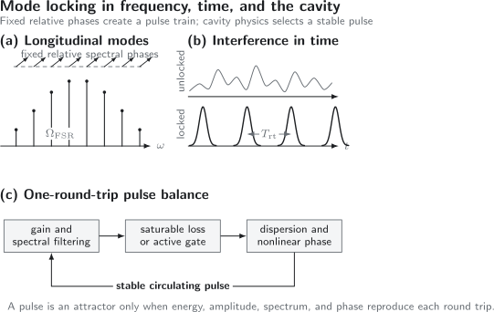
Three complementary views of mode locking. Fixed relative phases among longitudinal modes produce periodic constructive interference. A stable pulse additionally requires the combined gain, filtering, loss, dispersion, and nonlinear phase to reproduce its energy and complex envelope after each round trip.

Spectral Phase and Pulse Timing

Expand the spectral phase around $\omega_0$:

$$\phi(\omega_0+\Omega) = \phi_0 + \phi_1\Omega + \frac{\phi_2}{2}\Omega^2 + \frac{\phi_3}{6}\Omega^3 + \cdots.$$

Each coefficient has a distinct physical role.

Term	Effect on the pulse
$\phi_0$	overall carrier phase
$\phi_1$	envelope delay by $\phi_1$
$\phi_2$	group-delay dispersion and linear chirp
$\phi_3$	asymmetric distortion and higher-order chirp
higher orders	satellites, pedestals, and detailed waveform structure

The group delay is

$$t_g(\omega) = \frac{d\phi}{d\omega} = \phi_1+\phi_2\Omega+\frac{\phi_3}{2}\Omega^2+\cdots.$$

A transform-limited pulse has constant spectral phase up to the physically irrelevant affine terms. This is a stronger statement than saying that the spectrum is broad.

The carrier oscillation can also slip relative to the envelope from pulse to pulse because phase and group velocities are different. That carrier-envelope phase slip produces a carrier-envelope offset in the frequency-domain comb. Frequency Combs develops that metrological relation; here it is enough to note that ordinary intensity mode locking can be stable even when the absolute carrier-envelope phase is not stabilized.

Active Mode Locking

Active mode locking imposes a periodic modulation synchronized to the cavity. An electro-optic or acousto-optic element can modulate loss, amplitude, phase, frequency, or occasionally gain.

Amplitude modulation as a loss window

Suppose the round-trip transmission near a maximum is

$$M(\tau) \simeq \exp \left[ -\frac{1}{2} m\Omega_m^2\tau^2 \right],$$

where $m>0$ measures modulation depth and the origin is the least-loss time. Repeated round trips penalize field outside this window. Gain filtering penalizes excessive spectral width. Their competition admits a localized pulse, commonly close to Gaussian in the simplest linear active-locking model.

In the frequency domain, multiplication by a sinusoidal modulation mixes components separated by $\Omega_m$. Choosing

$$\Omega_m = p\Omega_{\rm FSR}, \qquad p\in\mathbb N,$$

couples cavity modes separated by $p$ mode indices. Fundamental mode locking uses $p=1$. Harmonic mode locking can produce $p$ equally spaced pulses per round trip and an output repetition frequency $p f_{\rm rep}$, although supermode competition and timing noise then require care.

Phase and frequency modulation

A phase modulator applies

$$\exp[i\beta_m\cos(\Omega_m t)],$$

which generates sidebands at integer multiples of $\Omega_m$ and couples longitudinal modes. In frequency-modulation mode locking, the circulating pulse may sit where the modulation-induced frequency sweep and cavity or gain filtering balance. Amplitude and frequency modulation therefore need not select identical pulse phases or chirps.

Synchronism and detuning

Write

$$\Omega_m = p\Omega_{\rm FSR} + \delta\Omega.$$

For $\delta\Omega\ne0$, the modulation window slips relative to the circulating pulse. Small detuning can shift the steady pulse time and add chirp; larger detuning destroys locking or produces unstable motion. A useful accumulated-slip estimate after $n$ round trips is

$$\Delta t_n \simeq nT_{\rm rt} \frac{\delta\Omega}{p\Omega_{\rm FSR}},$$

valid when the fractional mismatch is small. The locking range is not set by this kinematic estimate alone: modulation depth, gain bandwidth, cavity loss, dispersion, and pulse dynamics determine whether restoring forces can compensate the slip.

Active locking offers an externally referenced repetition rate and deterministic timing. It usually produces longer pulses than broadband passive femtosecond oscillators because available modulation and filtering strengths are finite, though hybrid systems combine active timing control with passive pulse shortening.

Passive Mode Locking

Passive mode locking uses intensity-dependent intracavity physics. A high-intensity fluctuation experiences lower effective loss or better gain overlap than a low-intensity background. Repetition of this discrimination can turn noise into a localized pulse.

Fast saturable absorber

A simple instantaneous loss model is

$$q(I) = q_{\rm ns} + \frac{\Delta q}{1+I/I_{\rm sat}},$$

where $q_{\rm ns}$ is nonsaturable loss, $\Delta q$ is modulation depth, and $I_{\rm sat}$ is a saturation scale. Since $q(I)$ decreases with intensity, the pulse peak sees less loss than its wings or a continuous-wave background.

“Fast” means that the absorber recovery time is short compared with the pulse duration or with the temporal structure being modeled. It does not mean that the device has zero recovery time in every experiment.

Slow saturable absorber

When recovery is not instantaneous, the absorber state needs its own dynamics. One schematic fluence-based model is

$$\frac{dq}{d\tau} = \frac{q_0-q}{\tau_a} - \frac{qI(\tau)}{E_{{\rm sat},a}},$$

where $\tau_a$ is the recovery time and $E_{{\rm sat},a}$ is a saturation energy per effective mode area. The leading edge bleaches the absorber and the recovery history affects the trailing edge and interpulse background. Fast and slow absorbers can support different pulse shapes and stability boundaries; substituting one algebraic model for the other can give qualitatively wrong predictions.

Semiconductor saturable-absorber mirrors

A semiconductor saturable-absorber mirror, or SESAM, combines a reflecting structure with engineered saturable absorption. Design variables include:

• modulation depth;
• saturation fluence;
• nonsaturable loss;
• recovery components;
• optical bandwidth;
• dispersion;
• damage and rollover fluence.

Too little modulation may not suppress continuous-wave operation. Too much modulation or an unfavorable ratio of gain and absorber saturation energies can favor Q-switched mode locking. A SESAM is therefore not simply an idealized transmission curve; its dynamics, mode area, thermal environment, and operating fluence matter.

Kerr-lens mode locking

An optical Kerr medium has

$$n = n_0+n_2 I.$$

The resulting self-focusing makes the intracavity spatial mode depend on instantaneous power. With a hard aperture, high-power portions can pass with lower diffraction loss. With a soft aperture, they can overlap the pumped gain region more efficiently. Either mechanism acts as an ultrafast effective saturable absorber.

Kerr-lens mode locking couples spatial and temporal dynamics. Cavity alignment, astigmatism, aperture position, pump-mode overlap, dispersion, and nonlinear phase all influence the operating state. A one-dimensional temporal model can explain pulse shaping after the effective saturable loss is known, but it cannot predict the complete alignment landscape.

Kerr-lens lasers can be difficult to self-start because the desired high-intensity state may coexist with a stable continuous-wave state. Mechanical perturbation, pump modulation, an additional absorber, or careful cavity design can seed the pulsed basin of attraction.

Nonlinear polarization evolution

In fibers, self- and cross-phase modulation change the polarization state in an intensity-dependent way. Wave plates, birefringent propagation, and a polarizer can convert that nonlinear polarization rotation into intensity-dependent transmission. This is often called nonlinear polarization evolution.

The mechanism can be fast and broadband, but its transfer function is periodic rather than a globally monotonic saturable absorber. Environmental birefringence, polarization drift, and non-polarization-maintaining components can make the operating point sensitive. An equivalent scalar loss model is useful only after the vector polarization dynamics have been reduced consistently.

The Round-Trip Master Equation

A mode-locked pulse is best regarded as a stable solution, often an attractor, of a round-trip map. Let $A(T,\tau)$ be the envelope, with $T$ varying slowly from round trip to round trip. A schematic Haus-type mean-field equation is

$$\begin{aligned} \frac{\partial A}{\partial T} ={}& \left[ g(E)-\ell-q(|A|^2) \right]A \\ &+ \left( D_f - i\frac{\beta_2}{2} \right) \frac{\partial^2 A}{\partial\tau^2} + i\gamma |A|^2A. \end{aligned}$$

Here

$$E = \int_{-\infty}^{\infty} |A(T,\tau)|^2\,d\tau$$

is proportional to pulse energy. A common gain-saturation model is

$$g(E) = \frac{g_0}{1+E/E_{{\rm sat},g}}.$$

The terms have clear roles:

Term	Round-trip role
$g(E)-\ell$	saturated gain versus unsaturable loss
$-q(	A
$D_f\partial_\tau^2A$	finite gain bandwidth or spectral filtering
$-i(\beta_2/2)\partial_\tau^2A$	net group-velocity dispersion
$i\gamma	A

The signs and normalizations vary across laser architectures. Some models need higher-order dispersion, self-steepening, Raman response, vector polarization, carrier dynamics, spatial diffraction, discrete components, or stochastic noise. The equation above is a structural model, not a universal law and not a quantum master equation for a density operator.

Fixed point and stability

If $\mathcal R$ denotes the exact complex round-trip map, a stationary mode-locked state obeys

$$A_*(\tau) = e^{i\theta} \mathcal R[A_*(\tau-\tau_0)].$$

The overall phase $\theta$ and time shift $\tau_0$ reflect symmetries. A physically observed state must also be stable: small perturbations in energy, timing, phase, spectrum, spatial mode, and polarization should decay or remain bounded. Finding a formal pulse solution without analyzing its perturbations is not enough to establish mode locking.

Pulse shaping is a balance

Several limiting pictures are useful:

• Active Gaussian pulses: a quadratic time gate balances spectral filtering.
• Saturable-absorber pulses: intensity discrimination suppresses the background and shortens the pulse until bandwidth, recovery, or other effects intervene.
• Soliton-like pulses: anomalous dispersion and self-phase modulation balance approximately, while gain and loss maintain the energy.
• Stretched pulses: the pulse broadens and compresses strongly around the cavity, reducing peak nonlinear phase in selected sections.
• Dissipative pulses: normal dispersion, nonlinearity, gain, loss, and spectral filtering jointly form a chirped attractor; dispersion and nonlinearity need not cancel point by point.

The shortest pulse is not always the most stable or highest-energy solution. Changing pump power can drive pulse splitting because one pulse cannot absorb additional gain without exceeding a nonlinear, absorber, or filtering stability boundary.

Pulse Duration and Bandwidth

Fourier convention

For an envelope $A(t)$, use the ordinary-frequency pair

$$\begin{aligned} \widetilde A(\nu) &= \int_{-\infty}^{\infty} A(t)e^{i2\pi\nu t}\,dt, \\ A(t) &= \int_{-\infty}^{\infty} \widetilde A(\nu)e^{-i2\pi\nu t}\,d\nu. \end{aligned}$$

The spectral intensity is proportional to $|\widetilde A(\nu)|^2$. A time–bandwidth product is meaningful only after specifying:

1. field or intensity profile;
2. FWHM, rms, or another width measure;
3. ordinary frequency $\nu$ or angular frequency $\omega$;
4. transform-limited or chirped phase;
5. whether pedestals and satellites are included.

Fourier Transform develops the transform machinery and Fourier Transform Conventions compares normalizations.

Gaussian transform limit

Take a Gaussian field envelope

$$A(t) = A_0 \exp \left( -\frac{t^2}{2\tau_0^2} \right).$$

Its intensity is

$$I(t) = I_0 \exp \left( -\frac{t^2}{\tau_0^2} \right),$$

with intensity FWHM

$$\Delta t = 2\sqrt{\ln2}\,\tau_0.$$

The Fourier amplitude and spectral intensity have the forms

$$\begin{aligned} \widetilde A(\nu) &\propto \exp \left( -2\pi^2\tau_0^2\nu^2 \right), \\ |\widetilde A(\nu)|^2 &\propto \exp \left( -4\pi^2\tau_0^2\nu^2 \right). \end{aligned}$$

Therefore

$$\Delta\nu = \frac{\sqrt{\ln2}}{\pi\tau_0},$$

and the transform-limited intensity-FWHM product is

$$\Delta\nu\,\Delta t = \frac{2\ln2}{\pi} \simeq 0.441.$$

Equality requires a Gaussian amplitude and affine spectral phase. For a $\operatorname{sech}^2$ intensity pulse,

$$I(t) = I_0 \operatorname{sech}^2 \left( \frac{t}{\tau_s} \right),$$

the transform-limited intensity-FWHM product is approximately

$$\Delta\nu\,\Delta t \simeq 0.315.$$

Using $0.441$ for every measured pulse silently assumes the answer. Real pulses can have asymmetry, spectral holes, satellite pulses, or phase structure for which one shape factor is inadequate.

Group-delay-dispersion broadening

For the Gaussian above, let a component add quadratic spectral phase

$$\widetilde A(\Omega) \longrightarrow \widetilde A(\Omega) \exp \left( i\frac{\phi_2}{2}\Omega^2 \right),$$

where $\Omega$ is angular-frequency offset and $\phi_2$ has units of time squared. The output intensity FWHM is

$$\Delta t = \Delta t_0 \sqrt{ 1+ \left( \frac{\phi_2}{\tau_0^2} \right)^2 }, \qquad \Delta t_0 = 2\sqrt{\ln2}\,\tau_0.$$

Equivalently,

$$\Delta t = \Delta t_0 \sqrt{ 1+ \left( \frac{4\ln2\,\phi_2}{\Delta t_0^2} \right)^2 }.$$

Quadratic phase preserves the ideal spectral intensity while broadening the temporal intensity. A spectrometer alone therefore cannot determine pulse duration. Optical windows, air, fibers, objectives, modulators, and the sample itself can all add enough group-delay dispersion to make the pulse at the interaction region much longer than the pulse at the laser output.

For broadband few-cycle pulses, third- and higher-order dispersion, frequency-dependent beam size, spatial chirp, pulse-front tilt, and nonlinear propagation may invalidate a scalar quadratic-phase model.

Energy, Average Power, and Peak Power

For one pulse per round trip,

$$E_p = \frac{P_{\rm avg}}{f_{\rm rep}}.$$

This identity is independent of pulse shape, provided $P_{\rm avg}$ is the time-averaged power in the pulse train and background power is negligible. Peak power does depend on shape.

For the Gaussian intensity convention above,

$$\begin{aligned} E_p &= \int_{-\infty}^{\infty} P_0e^{-t^2/\tau_0^2}\,dt \\ &= \frac{\sqrt{\pi}}{2\sqrt{\ln2}} P_0\Delta t \\ &\simeq 1.0645\,P_0\Delta t. \end{aligned}$$

Thus

$$P_0 \simeq 0.9394 \frac{E_p}{\Delta t}.$$

For a $\operatorname{sech}^2$ pulse,

$$E_p \simeq 1.135 P_0\Delta t, \qquad P_0 \simeq 0.881 \frac{E_p}{\Delta t}.$$

Peak irradiance additionally requires the spatial beam profile and area. Using $P_{\rm avg}/\Delta t$ as a peak power misses the repetition rate and can be wrong by many orders of magnitude.

Measuring a Mode-Locked Pulse

No single instrument establishes every property of a pulse train.

Repetition rate and average quantities

A fast photodiode and radio-frequency spectrum analyzer measure $f_{\rm rep}$, harmonics, sidebands, and low-frequency amplitude instabilities. An optical power meter gives $P_{\rm avg}$. These measurements do not resolve a femtosecond pulse shape directly; detector impulse response and electronic bandwidth are much slower.

An optical spectrum analyzer or spectrometer measures $|\widetilde A(\nu)|^2$. Combining a spectrum with an assumed transform-limited shape gives only a lower bound or model-dependent estimate of duration.

Intensity autocorrelation

A background-free second-order intensity autocorrelation is

$$A_I^{(2)}(\tau) = \int_{-\infty}^{\infty} I(t)I(t-\tau)\,dt.$$

For a Gaussian intensity profile,

$$\Delta t_{\rm AC} = \sqrt{2}\,\Delta t.$$

For a $\operatorname{sech}^2$ profile,

$$\Delta t_{\rm AC} \simeq 1.543\,\Delta t.$$

The deconvolution factor is therefore a model choice. An intensity autocorrelation is symmetric in delay and generally does not determine the spectral phase, temporal asymmetry, or a unique pulse shape. Interferometric autocorrelation adds carrier-fringe information but still has ambiguities and requires careful normalization.

Complete-field methods

Frequency-resolved optical gating, or FROG, records a nonlinear signal spectrum as a function of delay,

$$I_{\rm FROG}(\omega,\tau) = \left| \int_{-\infty}^{\infty} E_{\rm sig}(t,\tau) e^{i\omega t}\,dt \right|^2,$$

and retrieves a complex pulse consistent with the measured two-dimensional trace. Different nonlinear geometries define different signal fields and ambiguities.

Spectral phase interferometry for direct electric-field reconstruction, or SPIDER, uses spectral shearing interferometry to infer spectral-phase differences, which are integrated to reconstruct phase. FROG and SPIDER are not interchangeable black boxes: phase matching, calibration, dynamic range, spatial sampling, pulse-to-pulse stability, and retrieval residuals must be reported.

A defensible characterization compares at least:

• measured and reconstructed spectrum;
• pulse duration and width convention;
• spectral phase or chirp;
• retrieval or consistency error;
• repetition-rate and pulse-energy stability;
• measurement plane relative to the experiment.

Instabilities and Failure Modes

Q-switched mode locking

In Q-switched mode locking, a train of short pulses sits inside a much slower energy envelope. Gain stores energy over many round trips, then releases it in bursts. A radio-frequency spectrum shows sidebands around $f_{\rm rep}$ at the Q-switching frequency, and a slow photodiode shows the envelope.

This regime is not simply “stronger mode locking.” It reflects unstable energy exchange among gain, absorber, and intracavity pulse. Increasing pump power, changing mode area, reducing absorber modulation depth, or changing the ratio of saturation energies can move the stability boundary, but the correct remedy is architecture-specific.

Multiple pulsing

When one pulse cannot stably carry the available energy, the cavity may form two or more pulses per round trip. These can be widely separated, bound with a fixed separation, or drift. An optical spectrum can show interference fringes, but the fringe spacing alone does not identify a unique temporal state without phase information.

Spectral and temporal side structure

Dispersion perturbations, resonant sidebands, gain filtering, self-phase modulation, etalons, and higher-order phase can produce spectral sidebands, temporal pedestals, or satellite pulses. A narrow autocorrelation central feature may coexist with substantial energy in a broad pedestal, which matters for nonlinear excitation and damage.

Timing and phase noise

Pulse timing jitter, carrier-envelope phase noise, optical-frequency noise, and relative intensity noise are distinct stochastic degrees of freedom. They can couple through dispersion, nonlinear phase, amplitude–phase conversion, and feedback. A narrow radio-frequency repetition-rate line does not by itself prove narrow optical comb teeth or a stable carrier-envelope phase.

Practical signatures

Observation	Plausible causes to test
slow envelope on pulse train	Q-switched mode locking, pump noise
two pulses per round trip	harmonic locking or pulse splitting
RF sidebands	timing modulation, Q switching, supermode beating
spectral fringes	multiple pulses, etalon, coherent reflection
broad pedestal	uncompensated phase, unstable pulses, amplifier effects
intermittent cw breakthrough	insufficient intensity discrimination
sudden spectral narrowing	loss of mode locking or reduced gain bandwidth
power rises while pulse shortens unexpectedly	measurement-plane or deconvolution error

Diagnosis should combine optical spectrum, radio-frequency spectrum, time-domain detector traces, autocorrelation or field retrieval, and average power. One trace rarely distinguishes all alternatives.

Connection to Ultrafast Spectroscopy

A mode-locked laser supplies a reproducible clock and a short interaction window. It does not automatically set the experiment’s time resolution.

Pump–probe response

For Gaussian pump and probe intensities with FWHM durations $\Delta t_p$ and $\Delta t_{\rm pr}$, an ideal instantaneous cross-correlation has

$$\Delta t_{\rm cc} = \sqrt{ \Delta t_p^2 + \Delta t_{\rm pr}^2 }.$$

The measured signal also convolves this instrument response with material dynamics, detector response, phase matching, propagation, and any timing jitter. A fitted time constant below the independently measured instrument response requires a model that justifies how it was inferred.

Characterize at the sample

The relevant pulse is the pulse where it interacts with matter. Before the sample, measure or calculate:

• dispersion of windows, objectives, fibers, modulators, and air;
• pulse-front tilt and spatial chirp;
• pump and probe spot sizes and overlap;
• pulse energy, peak irradiance, and repetition rate;
• polarization and incidence geometry;
• timing jitter and delay-stage calibration.

Compression optimized at the laser output can be wrong at the sample. Likewise, a pulse retrieved from one spatial point can miss space–time coupling elsewhere in the beam.

Perturbation, nonlinearity, and heating

Increasing peak intensity improves some nonlinear signal levels but can also drive multiphoton excitation, ionization, AC Stark shifts, saturation, coherent artifacts, or damage. Increasing repetition rate raises average heating and can prevent relaxation between pulses even at fixed pulse energy. A trustworthy experiment therefore reports both pulse energy and average power, along with beam area and sample conditions.

For few-cycle waveforms, the carrier-envelope phase can control subcycle strong-field dynamics. For many-cycle intensity-based pump–probe experiments, the envelope delay and spectral phase may be the dominant quantities. Whether carrier-envelope stabilization matters is an observable-dependent question, not a universal property of “ultrafast” work.

Ultrafast Spectroscopy Overview develops pump–probe, multidimensional, and nonlinear-spectroscopy applications without duplicating the laser-formation physics here.

An Analysis Workflow

1. Identify the cavity clock. Determine $T_{\rm rt}$, $f_{\rm rep}$, and whether operation is fundamental or harmonic.
2. Measure the optical spectrum. Record usable coherent bandwidth and look for filtering, fringes, sidebands, and clipping.
3. State the locking mechanism. Name the active gate, absorber, Kerr lens, polarization element, or hybrid mechanism and its relevant response time.
4. Write the round-trip balance. Include gain saturation, loss, filtering, dispersion, nonlinear phase, and any spatial or vector dynamics needed by the architecture.
5. Separate amplitude and phase. A broad spectrum does not determine a short pulse until spectral phase is known.
6. Characterize the pulse. Report duration convention, shape assumption or retrieved field, pulse energy, and measurement plane.
7. Test stability. Inspect slow time traces, radio-frequency spectra, pulse-to-pulse energy, and long records for multiple states.
8. Propagate to the experiment. Account for dispersion, nonlinearity, spatial coupling, and timing after the oscillator.

Common Mistakes

• Many modes imply mode locking. They do not; stable relative phase is essential.
• Locked means all phases are zero. An affine spectral phase only changes carrier phase and pulse arrival time.
• Pulse period equals pulse duration. Mode spacing sets the period; coherent bandwidth and phase set duration.
• Gain bandwidth equals pulse bandwidth. Intracavity loss, filtering, dispersion, and nonlinear dynamics usually narrow or reshape it.
• A broad spectrum proves a short pulse. Quadratic and higher spectral phase can strongly broaden the pulse without changing its spectrum.
• Every autocorrelation uses the same deconvolution factor. The factor depends on pulse shape and measurement type.
• Average power divided by pulse width is peak power. The repetition rate and pulse-shape factor are missing.
• A master-equation solution is automatically stable. Perturbation eigenvalues or time-domain evolution must support that claim.
• A clean autocorrelation excludes pedestals. Limited dynamic range can hide substantial low-intensity energy.
• Oscillator output characterizes the sample pulse. Downstream dispersion and space–time coupling can dominate.
• Mode locking stabilizes every comb degree of freedom. Timing, carrier-envelope phase, optical phase, and amplitude noise remain distinct.

Exercises

1. Equal-mode pulse train

Consider $M=2N+1$ modes with equal amplitude $A_0$, frequencies $\omega_0+m\Omega$, and equal phase at $t=0$.

Derive the Dirichlet-kernel envelope, find the pulse-train period, and compare the peak and period-averaged intensity scalings with $M$.

Solution

Factoring out the carrier gives

$$A(t) = A_0 \sum_{m=-N}^{N} e^{-im\Omega t}.$$

Use the finite geometric sum:

$$\begin{aligned} \sum_{m=-N}^{N}e^{-imx} &= e^{iNx} \frac{1-e^{-iMx}}{1-e^{-ix}} \\ &= \frac{\sin(Mx/2)}{\sin(x/2)}. \end{aligned}$$

With $x=\Omega t$,

$$A(t) = A_0 \frac{\sin(M\Omega t/2)}{\sin(\Omega t/2)}.$$

It is periodic with $T=2\pi/\Omega$. At $t=\ell T$, its limiting amplitude is $MA_0$, so $I_{\rm peak}\propto M^2|A_0|^2$. Over one period, orthogonality removes cross terms:

$$\langle I\rangle \propto \sum_{m=-N}^{N}|A_0|^2 = M|A_0|^2.$$

The peak-to-average ratio therefore scales as $M$.

2. Affine spectral phase

The modal phase is $\phi_m=\phi_0+m\phi_1$. Show that this phase pattern does not broaden the pulse. Find its time shift.

Solution

The envelope is

$$\begin{aligned} A(t) &= e^{i\phi_0} \sum_m a_m e^{-im(\Omega t-\phi_1)} \\ &= e^{i\phi_0} A_{\rm zero} \left( t-\frac{\phi_1}{\Omega} \right), \end{aligned}$$

where $A_{\rm zero}(t)$ is the envelope with zero modal phase. The intensity is shifted by

$$t_0 = \frac{\phi_1}{\Omega}$$

and otherwise unchanged. The constant $\phi_0$ changes only the overall field phase. Pulse broadening requires nonlinear spectral phase.

3. Gaussian time–bandwidth product

For

$$A(t)=A_0e^{-t^2/(2\tau_0^2)},$$

derive the intensity FWHM in time and ordinary frequency. Verify the transform-limited product.

Solution

The intensity is

$$I(t) = I_0e^{-t^2/\tau_0^2}.$$

Setting $I(t)=I_0/2$ gives

$$\Delta t = 2\tau_0\sqrt{\ln2}.$$

With the ordinary-frequency Fourier convention,

$$|\widetilde A(\nu)|^2 \propto e^{-4\pi^2\tau_0^2\nu^2}.$$

The half-maximum points obey $4\pi^2\tau_0^2\nu^2=\ln2$, hence

$$\Delta\nu = \frac{\sqrt{\ln2}}{\pi\tau_0}.$$

Multiplication gives

$$\Delta\nu\,\Delta t = \frac{2\ln2}{\pi} \simeq 0.441.$$

4. Broadening by group-delay dispersion

A transform-limited Gaussian has $\Delta t_0=30\,{\rm fs}$. It acquires $\phi_2=500\,{\rm fs}^2$. Using the Gaussian convention on this page, find the output FWHM.

Solution

First,

$$\tau_0 = \frac{\Delta t_0}{2\sqrt{\ln2}} \simeq 18.02\,{\rm fs}.$$

Then

$$\frac{\phi_2}{\tau_0^2} \simeq \frac{500}{(18.02)^2} \simeq 1.54.$$

Therefore

$$\begin{aligned} \Delta t &= 30\,{\rm fs} \sqrt{1+(1.54)^2} \\ &\simeq 55.1\,{\rm fs}. \end{aligned}$$

The spectral intensity is unchanged in the ideal quadratic-phase model, so a spectrometer alone would not reveal this broadening.

5. From average power to peak power

A fundamentally mode-locked laser has $P_{\rm avg}=500\,{\rm mW}$, $f_{\rm rep}=100\,{\rm MHz}$, and Gaussian intensity FWHM $\Delta t=100\,{\rm fs}$. Find the pulse energy and peak power.

Solution

The pulse energy is

$$E_p = \frac{0.500\,{\rm W}}{1.00\times10^8\,{\rm s}^{-1}} = 5.00\,{\rm nJ}.$$

For a Gaussian,

$$P_0 = 0.9394 \frac{E_p}{\Delta t}.$$

Thus

$$\begin{aligned} P_0 &= 0.9394 \frac{5.00\times10^{-9}\,{\rm J}} {100\times10^{-15}\,{\rm s}} \\ &\simeq 4.70\times10^4\,{\rm W}. \end{aligned}$$

The peak power is about $47\,{\rm kW}$. Peak irradiance still requires the beam area.

6. Active-locking mismatch

An active modulator is intended to operate at the fundamental repetition frequency $f_{\rm rep}=100\,{\rm MHz}$ but is high by $10\,{\rm Hz}$. Estimate the relative timing slip accumulated after $1\,{\rm ms}$ if no locking force corrects it.

Solution

The fractional frequency mismatch is

$$\frac{\delta f}{f_{\rm rep}} = 10^{-7}.$$

After elapsed time $t$, the relative slip is approximately

$$\Delta t \simeq t\frac{\delta f}{f_{\rm rep}}.$$

For $t=1\,{\rm ms}$,

$$\Delta t \simeq 10^{-3}\times10^{-7}\,{\rm s} = 100\,{\rm ps}.$$

This is a kinematic open-loop estimate. In a locked laser, modulation depth and pulse dynamics provide a finite restoring range; outside that range the pulse slips or locking fails.

7. Autocorrelation ambiguity

An intensity autocorrelation has FWHM $150\,{\rm fs}$. Infer the pulse FWHM assuming first a Gaussian pulse and then a $\operatorname{sech}^2$ pulse. Explain why the trace alone does not choose between them.

Solution

For a Gaussian,

$$\Delta t_{\rm G} = \frac{150\,{\rm fs}}{\sqrt2} \simeq 106\,{\rm fs}.$$

For a $\operatorname{sech}^2$ pulse,

$$\Delta t_{\rm sech} = \frac{150\,{\rm fs}}{1.543} \simeq 97.2\,{\rm fs}.$$

An intensity autocorrelation is an integral projection. Different pulse shapes and spectral phases can produce similar or identical traces, and the trace is symmetric even for an asymmetric pulse. Independent spectral information and a phase-sensitive retrieval such as FROG or SPIDER are needed to test the assumed shape.

8. Diagnose an unstable pulse train

A laser has a clean optical spectrum and a narrow autocorrelation central peak, but a slow photodiode shows bursts at $40\,{\rm kHz}$. The radio-frequency spectrum has sidebands at $f_{\rm rep}\pm40\,{\rm kHz}$. What is the leading diagnosis, and what additional measurements would you make?

Solution

The leading diagnosis is Q-switched mode locking: short pulses remain within a slowly modulated energy envelope. The clean single-shot or averaged optical measurements do not exclude slow pulse-energy instability.

Useful checks are:

1. a long time-domain trace resolving many $40\,{\rm kHz}$ periods;
2. radio-frequency spectra around several harmonics and near dc;
3. pulse-energy statistics or a fast photodiode histogram;
4. pump-power and absorber-fluence dependence;
5. autocorrelation or field retrieval triggered at different points in the slow envelope;
6. a check for multiple pulses per cavity round trip.

The result should not be called stable continuous-wave mode locking until the slow envelope and sidebands are removed or quantitatively bounded.

References

1. L. E. Hargrove, R. L. Fork, and M. A. Pollack, “Locking of He–Ne laser modes induced by synchronous intracavity modulation,” Applied Physics Letters 5, 4–5 (1964), doi:10.1063/1.1754025.
2. D. J. Kuizenga and A. E. Siegman, “FM and AM mode locking of the homogeneous laser, Part I: Theory,” IEEE Journal of Quantum Electronics 6, 694–708 (1970), doi:10.1109/JQE.1970.1076343.
3. D. J. Kuizenga and A. E. Siegman, “FM and AM mode locking of the homogeneous laser, Part II: Experimental results in a Nd:YAG laser with internal FM modulation,” IEEE Journal of Quantum Electronics 6, 709–715 (1970), doi:10.1109/JQE.1970.1076344.
4. A. Dienes, E. P. Ippen, and C. V. Shank, “A mode-locked cw dye laser,” Applied Physics Letters 19, 258–260 (1971), doi:10.1063/1.1653909.
5. E. P. Ippen, C. V. Shank, and A. Dienes, “Passive mode locking of the cw dye laser,” Applied Physics Letters 21, 348–350 (1972), doi:10.1063/1.1654406.
6. H. A. Haus, “Theory of mode locking with a fast saturable absorber,” Journal of Applied Physics 46, 3049–3058 (1975), doi:10.1063/1.321997.
7. H. A. Haus, “Theory of mode locking with a slow saturable absorber,” IEEE Journal of Quantum Electronics 11, 736–746 (1975), doi:10.1109/JQE.1975.1068922.
8. D. E. Spence, P. N. Kean, and W. Sibbett, “60-fsec pulse generation from a self-mode-locked Ti:sapphire laser,” Optics Letters 16, 42–44 (1991), doi:10.1364/OL.16.000042.
9. U. Keller et al., “Semiconductor saturable absorber mirrors (SESAMs) for femtosecond to nanosecond pulse generation in solid-state lasers,” IEEE Journal of Selected Topics in Quantum Electronics 2, 435–453 (1996), doi:10.1109/2944.571743.
10. H. A. Haus, “Mode-locking of lasers,” IEEE Journal of Selected Topics in Quantum Electronics 6, 1173–1185 (2000), doi:10.1109/2944.902165.
11. A. Chong, J. Buckley, W. Renninger, and F. Wise, “All-normal-dispersion femtosecond fiber laser,” Optics Express 14, 10095–10100 (2006), doi:10.1364/OE.14.010095.
12. D. J. Kane and R. Trebino, “Characterization of arbitrary femtosecond pulses using frequency-resolved optical gating,” IEEE Journal of Quantum Electronics 29, 571–579 (1993), doi:10.1109/3.199311.
13. C. Iaconis and I. A. Walmsley, “Spectral phase interferometry for direct electric-field reconstruction of ultrashort optical pulses,” Optics Letters 23, 792–794 (1998), doi:10.1364/OL.23.000792.
14. A. E. Siegman, Lasers (University Science Books, 1986), Chapters 27–28.
15. J.-C. Diels and W. Rudolph, Ultrashort Laser Pulse Phenomena, 2nd ed. (Academic Press, 2006).
16. A. M. Weiner, Ultrafast Optics (Wiley, 2009), doi:10.1002/9780470473467.

Further Connections

• Lasers Overview
• Laser Principles
• Optical Cavities
• Laser Modes
• Linewidth and Coherence
• Nonlinear Quantum Optics
• Ultrafast Spectroscopy Overview
• Fourier Transform
• Wave Packets

Frontier Context

Attosecond and Ultrafast Frontiers tracks dated evidence and open questions in isolated attosecond sources, high-harmonic emission, field-resolved metrology, and strong-field control. The mode-comb picture, pulse-formation mechanisms, bandwidth limits, chirp, stability, and optical diagnostics developed here remain canonical.