Gain and Threshold

Laser threshold is the operating point at which the leading self-consistent cavity mode changes from net decay to net small-signal growth. The word leading matters. A gain medium does not reach threshold in the abstract; a particular spatial, spectral, and polarization mode reaches it after sampling a particular pump distribution and a particular loss budget.

The cleanest bookkeeping variable is the logarithmic round-trip power margin

$$\mathcal M_\mu \equiv \ln \mathcal G_{\mathrm{rt},\mu},$$

where $\mu$ labels a complete candidate cavity mode and $\mathcal G_{\mathrm{rt},\mu}$ is its round-trip power multiplier in the small-signal limit. Then

$$\begin{array}{ccl} \mathcal M_\mu<0 &:& \text{mode decays}, \\ \mathcal M_\mu=0 &:& \text{mode is at threshold}, \\ \mathcal M_\mu>0 &:& \text{mode initially grows}. \end{array}$$

Logs turn multiplicative mirror transmissions, aperture survivals, and propagation factors into one additive audit trail. They also expose most factor-of-two errors.

Canonical Scope

This page owns the quantitative threshold layer:

1. material, modal, local, integrated, and logarithmic gain;
2. distributed absorption, scattering, diffraction, mirror, aperture, and output-coupling losses;
3. exact linear-cavity and ring-cavity round-trip conditions;
4. threshold as the largest round-trip eigenvalue reaching unit magnitude;
5. spectral and transverse mode competition at onset;
6. translations among round-trip loss, photon lifetime, decay rate, cavity linewidth, and quality factor;
7. saturation and gain clamping beyond onset;
8. operational threshold definitions for conventional and high-$\beta$ lasers;
9. uncertainty and sensitivity checks for a measured loss budget.

Laser Principles owns the first nonlinear round-trip map and the basic output-coupling tradeoff. Population Inversion owns the pumping cycles that create material gain. Stimulated Emission owns microscopic cross sections and gain saturation.

This page extends those results to nonuniform modal bookkeeping. Rate-Equation Lasers derives the population and photon dynamics after a mode has been selected. Optical Cavities owns passive resonator geometry, lifetime, spectral response, and spatial stability. Laser Modes owns normalized transverse eigenfunctions, degeneracy, beam quality, and competition beyond onset. Linewidth and Coherence and Mode Locking own the corresponding phase-noise and multimode pulse dynamics.

Convention Ledger

Use:

• $g_{\mathrm{mat}}(\mathbf r,\omega)$ for a local material power-gain coefficient in $\mathrm{m}^{-1}$;
• $\Gamma_\mu(\mathbf r)$ for the local weighting or overlap of mode $\mu$ with active material;
• $\alpha_\mu(\mathbf r)$ for local distributed power loss;
• $R_j$, $T_j$, and $A_j$ for mirror power reflection, useful transmission, and parasitic absorption or scattering;
• $\ell_{\mu j}$ for other lumped power survival factors;
• $\mathcal G_{\mathrm{rt},\mu}$ for a round-trip power multiplier;
• $\mathcal M_\mu=\ln\mathcal G_{\mathrm{rt},\mu}$ for its logarithmic margin;
• $t_{\mathrm{rt}}$ for round-trip group delay;
• $\kappa$ for stored-energy decay rate, so $U(t)=U(0)e^{-\kappa t}$;
• $Q=\omega/\kappa$ for the cold-cavity quality factor under that convention;
• $\Delta\nu_{\mathrm c}$ for cold-cavity power-spectrum FWHM in Hz.

With these choices,

$$\Delta\nu_{\mathrm c} = \frac{\kappa}{2\pi}, \qquad Q = \frac{\nu}{\Delta\nu_{\mathrm c}}.$$

Some references use $\kappa$ for field-amplitude decay, making energy decay $2\kappa$. Translate the defining differential equation before comparing formulas.

Gain Coefficients

For a weak traveling wave,

$$\frac{dI}{dz} = \left[ g_{\mathrm{mat}}(z,\omega) - \alpha(z,\omega) \right]I.$$

Integrating makes the additive gain and loss budget explicit:

$$\begin{aligned} \ln\frac{I(z_2)}{I(z_1)} ={}& \int_{z_1}^{z_2} g_{\mathrm{mat}}(z,\omega)\,dz \\ &- \int_{z_1}^{z_2} \alpha(z,\omega)\,dz . \end{aligned}$$

Both integrals are dimensionless; exponentiating their difference gives the power ratio.

Material versus modal gain

A cavity mode samples only the component of gain overlapping its field, polarization, frequency, and pumped region. In a simple scalar reduction,

$$g_\mu(z,\omega) = \Gamma_\mu(z) g_{\mathrm{mat}}(z,\omega),$$

with $0\le\Gamma_\mu\le1$. More generally, gain is a tensor and the weighting is an overlap integral over the transverse field and active susceptibility.

For transverse mode profile $u_\mu(x,y;z)$ normalized at each $z$, one useful power weighting is

$$\Gamma_\mu(z) = \frac{ \displaystyle \int_{\mathrm{active}} |u_\mu(x,y;z)|^2\,dx\,dy }{ \displaystyle \int_{\mathrm{all}} |u_\mu(x,y;z)|^2\,dx\,dy }.$$

If gain varies transversely, replacing it by $\Gamma_\mu g_{\mathrm{mat}}$ is valid only when the chosen average is stated. The more general modal gain is an intensity-weighted integral of the local gain.

Local, integrated, and dimensionless gain

These phrases should not be interchanged:

Quantity	Definition	Units
gain coefficient	$g_\mu(z)$	$\mathrm{m}^{-1}$
integrated gain exponent	$\int g_\mu dz$	dimensionless
power gain	$G=\exp(\int g_\mu dz)$	dimensionless
gain in decibels	$10\log_{10}G$	dB

For natural-log power margin $\mathcal M$,

$$\mathcal M_{\mathrm{dB}} = \frac{10}{\ln10}\mathcal M \simeq 4.343\mathcal M.$$

Threshold corresponds to zero net dB per round trip, not zero material gain.

Gain spectrum

The local gain inherits:

• homogeneous and inhomogeneous line shapes;
• upper and lower sublevel populations;
• polarization selection rules;
• pump-induced Stark, Zeeman, thermal, and carrier shifts;
• reabsorption and excited-state absorption;
• dispersion linked to the complex susceptibility.

A peak-gain number without wavelength, temperature, polarization, and small-signal conditions is not a complete material specification.

Loss Budget

Loss is every process that removes energy from the candidate intracavity mode over one round trip.

Distributed loss

Distributed loss may include:

• background absorption in the gain host, gas, windows, or coatings;
• scattering from inhomogeneity, surfaces, particles, or defects;
• waveguide propagation loss;
• diffraction or radiation leakage represented locally;
• free-carrier or excited-state absorption.

For nonuniform $\alpha_\mu(s)$, its round-trip logarithmic contribution is

$$\mathcal L_{\mathrm{dist},\mu} = \oint \alpha_\mu(s)\,ds.$$

This is positive in a loss budget and enters the round-trip margin with a minus sign.

Lumped loss

If an element transmits a fraction $\ell_j$ of mode power per encounter, its logarithmic loss is

$$\mathcal L_j = -\ln\ell_j \ge 0.$$

For several independent elements,

$$\ell_{\mathrm{rt}} = \prod_j\ell_j,$$

and

$$-\ln\ell_{\mathrm{rt}} = \sum_j \left( -\ln\ell_j \right).$$

Percent losses add only approximately. Logarithmic losses add exactly.

Mirrors and output coupling

For a linear two-mirror cavity, the round-trip mirror survival is

$$R_1R_2.$$

The exact equivalent mirror-loss coefficient referred to a gain path of one-way length $L$ is

$$\alpha_{\mathrm m} = \frac{1}{2L} \ln \left( \frac{1}{R_1R_2} \right).$$

This equivalent coefficient is a bookkeeping device. Mirror loss remains lumped at physical surfaces.

If mirror 2 obeys

$$R_2+T_2+A_2 = 1,$$

then both useful transmission $T_2$ and parasitic loss $A_2$ raise threshold. Only $T_2$ produces the intended output.

Small-loss approximation

For $x\ll1$,

$$-\ln(1-x) = x + \frac{x^2}{2} + \cdots.$$

Thus a mirror with total nonreflection $1-R\ll1$ contributes approximately $1-R$ to round-trip fractional loss. The approximation is often adequate, but the exact logarithm is just as easy and remains reliable at larger loss.

Diffraction and mode mismatch

Diffraction loss is mode dependent. An aperture may transmit the fundamental mode efficiently while strongly attenuating a higher-order transverse mode. Likewise, an intracavity filter or birefringent element can give different loss to nearby frequencies or polarizations.

There is therefore no universal scalar “cavity loss” independent of the mode. A threshold calculation must carry an index $\mu$ whenever competing modes sample different losses.

Exact Round-Trip Margins

Uniform linear cavity

For a gain region of one-way length $L$ traversed twice, mirror reflectivities $R_{1\mu}$ and $R_{2\mu}$, and additional round-trip lumped survival $\ell_\mu$,

$$\begin{aligned} \mathcal M_\mu ={}& \ln\ell_\mu + \ln R_{1\mu} + \ln R_{2\mu} \\ &+ 2 \int_0^L \Gamma_\mu(z) g_{\mathrm{mat}}(z,\omega_\mu)\,dz \\ &- 2 \int_0^L \alpha_\mu(z) \,dz . \end{aligned}$$

Every factor is a power quantity and every event is counted once per complete round trip.

For uniform coefficients,

$$\begin{aligned} \mathcal M_\mu ={}& \ln \left( \ell_\mu R_{1\mu} R_{2\mu} \right) \\ &+ 2L \left( \Gamma_\mu g_{\mathrm{mat},\mu} - \alpha_\mu \right). \end{aligned}$$

Ring cavity

For a traveling-wave ring with one circuit $\mathcal C$,

$$\begin{aligned} \mathcal M_\mu ={}& \ln\ell_\mu \\ &+ \oint_{\mathcal C} \Gamma_\mu(s) g_{\mathrm{mat}}(s,\omega_\mu)\,ds \\ &- \oint_{\mathcal C} \alpha_\mu(s) \,ds . \end{aligned}$$

The active section is counted once per circuit unless the actual optical path passes it more than once. Importing the linear-cavity factor of two into a single-pass ring is a common threshold error.

Field-amplitude form

If the complex field returns as

$$\mathcal E_{m+1} = \lambda_\mu\mathcal E_m,$$

then

$$\mathcal G_{\mathrm{rt},\mu} = |\lambda_\mu|^2, \qquad \mathcal M_\mu = 2\ln|\lambda_\mu|.$$

Threshold is $|\lambda_\mu|=1$, equivalent to $\mathcal G_{\mathrm{rt},\mu}=1$. Mixing a field eigenvalue with a power reflectivity creates a factor-of-two error.

Phase and Modal Self-Consistency

Magnitude balance is imposed only on candidate modes that reproduce their field profile and phase after a round trip. In a simple scalar cavity,

$$\Phi_{\mathrm{rt},\mu} = 2\pi q.$$

In a general open resonator, propagation through gain, loss, apertures, mirrors, waveguides, and polarization elements defines a nonunitary round-trip operator $\mathcal R$:

$$\mathcal R u_\mu = \lambda_\mu u_\mu.$$

Both the eigenfunction $u_\mu$ and eigenvalue $\lambda_\mu$ can depend on pump through gain guiding, thermal lensing, carrier-induced index, and saturation. The cold-cavity mode is often a starting approximation, not an immutable field shape.

First Threshold and Mode Competition

Among all self-consistent candidate modes, first threshold occurs when

$$\max_\mu \mathcal M_\mu = 0.$$

The first lasing mode is

$$\mu_* = \operatorname*{arg\,max}_\mu \mathcal M_\mu.$$

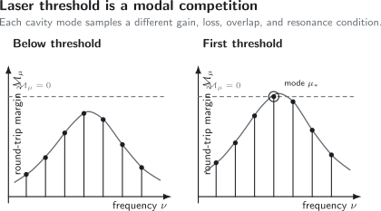
Threshold is reached by a complete cavity mode, not by the gain-envelope maximum alone. Discrete resonances sample different gain, loss, spatial overlap, and polarization response. As pump rises, the leading modal round-trip margin reaches zero first; later saturation and cross-saturation can reorder the competition.

The mode nearest peak material gain need not win. Another mode can have:

• better overlap with the pumped volume;
• lower diffraction or mirror loss;
• a favored polarization;
• lower reabsorption;
• a resonance shifted by gain dispersion;
• less competition from already occupied modes.

Uniform threshold gain

For the uniform linear model, setting $\mathcal M_\mu=0$ gives

$$\begin{aligned} \Gamma_\mu g_{\mathrm{mat,th},\mu} ={}& \alpha_\mu \\ &+ \frac{1}{2L} \ln \left[ \frac{1}{ \ell_\mu R_{1\mu} R_{2\mu} } \right]. \end{aligned}$$

Therefore

$$\begin{aligned} g_{\mathrm{mat,th},\mu} ={}& \frac{1}{\Gamma_\mu} \Bigg\{ \alpha_\mu \\ &+ \frac{1}{2L} \ln \left[ \frac{1}{ \ell_\mu R_{1\mu} R_{2\mu} } \right] \Bigg\}. \end{aligned}$$

Poor overlap raises the required material gain even though the cavity loss itself is unchanged.

Threshold inversion

If a declared transition obeys

$$g_{\mathrm{mat}} = \sigma \Delta\mathcal N$$

under equal-cross-section assumptions, then

$$\Delta\mathcal N_{\mathrm{th}} = \frac{ g_{\mathrm{mat,th}} }{ \sigma }.$$

For unequal absorption and emission cross sections, solve

$$\sigma_e\mathcal N_u - \sigma_a\mathcal N_l = g_{\mathrm{mat,th}}$$

with the actual population constraints. Converting that population to pump power belongs to the population and rate-equation model.

Photon Lifetime, Cavity Linewidth, and Q

Turn off gain and let stored cavity energy obey

$$\frac{dU}{dt} = -\kappa U.$$

Over one round-trip time,

$$\frac{ U(t+t_{\mathrm{rt}}) }{ U(t) } = e^{-\kappa t_{\mathrm{rt}}}.$$

The cold-cavity logarithmic round-trip loss is therefore

$$\mathcal L_{\mathrm{rt}} = \kappa t_{\mathrm{rt}}.$$

If a uniformly averaged modal gain coefficient $\bar g_\mu$ acts around a path with group velocity $v_g$, its power-growth rate is $v_g\bar g_\mu$. Threshold becomes

$$v_g \bar g_{\mathrm{th}} = \kappa.$$

For localized gain,

$$\bar g_\mu = \frac{1}{L_{\mathrm{rt}}} \oint \Gamma_\mu(s) g_{\mathrm{mat}}(s)\,ds$$

when $v_g$ can be treated as uniform. Strong dispersion requires the group delay and energy normalization to be handled more carefully.

With the energy-decay convention,

$$Q = \frac{\omega}{\kappa}, \qquad \Delta\nu_{\mathrm c} = \frac{\kappa}{2\pi}.$$

A high $Q$ reduces passive decay but does not by itself guarantee low pump threshold. Small mode volume, pump overlap, reabsorption, nonradiative processes, and spontaneous-emission coupling also matter.

Saturation Above Threshold

The threshold calculation uses small-signal gain. Above threshold, the oscillating field changes the population and hence the gain.

For a local saturation model,

$$g_{\mathrm{mat}} \left( \mathbf r,I_\mu \right) = \frac{ g_0(\mathbf r) }{ 1+ I_\mu(\mathbf r)/ I_{\mathrm{sat}}(\mathbf r) }.$$

The steady single-mode condition is the nonlinear integrated balance

$$\mathcal M_\mu \left[ I_\mu(\mathbf r) \right] = 0.$$

This means the complete saturated round-trip gain balances loss. It does not mean:

• $g(\mathbf r)=g_{\mathrm{th}}$ at every point;
• all frequencies are clamped to threshold;
• every competing mode sees zero margin;
• unsampled parts of an inhomogeneous ensemble are saturated.

Spatial hole burning

In a standing-wave cavity, intensity nodes and antinodes saturate the medium unequally. Unsaturated inversion can remain near nodes. Another longitudinal mode with a shifted standing-wave pattern can draw on that residual gain, weakening homogeneous mode competition.

Spectral hole burning

In an inhomogeneously broadened medium, one narrow mode saturates mainly the resonant subensemble. Other frequency classes retain gain and can support additional longitudinal modes.

Gain clamping and pump increase

For a simple homogeneous single-mode laser, increasing pump above threshold mainly raises photon number and useful output while the saturated modal gain stays near threshold. In spatially structured or multimode systems, local inversion and nonlasing-mode margins can continue to change substantially.

Experimental Threshold

The linear-stability threshold is mathematically precise inside a declared model. A finite noisy experiment may not display one uniquely sharp point.

Light–light curve

Plot output power versus absorbed pump power. A conventional low-$\beta$ laser often shows:

• spontaneous output below threshold;
• a transition region;
• an approximately linear stimulated-output branch above threshold.

Fitting two straight lines and intersecting them is an operational convention, not a universal theorem. Background subtraction, detector saturation, pump absorption, thermal drift, and changing collection efficiency affect the result.

Spectral and coherence signatures

Useful corroborating changes include:

• emergence of one or more resonator-defined peaks;
• spectral narrowing;
• increasing first-order coherence time;
• photon statistics evolving from thermal-like toward laser-like behavior;
• gain clamping or inversion changes;
• relaxation-oscillation signatures.

No one signature is sufficient in every architecture. Narrow spontaneous or amplified emission can mimic a spectral peak, and passive filtering can produce a narrow spectrum without oscillation.

High-β and small lasers

Let $\beta$ be the fraction of spontaneous emission coupled into the selected laser mode. In conventional macroscopic lasers, $\beta\ll1$, and the stimulated branch can dominate abruptly. In micro- and nanolasers with large $\beta$, spontaneous emission already feeds the selected mode strongly and the input–output kink can become weak or disappear.

Threshold then requires joint evidence from photon statistics, coherence, spectra, and a validated dynamical model. The phrase “thresholdless laser” usually means a smooth light–light curve or $\beta$ near one, not absence of loss, saturation, or a coherence crossover.

Hysteresis and multiple thresholds

Thermal effects, saturable absorption, optical bistability, mode hopping, and nonlinear feedback can give different turn-on and turn-off pump values. Report the scan direction, speed, initial state, and dwell time. A single threshold number can conceal real dynamics.

Worked Loss-Budget Audit

Consider a uniform linear cavity with

$$\begin{gathered} L=0.400\ \mathrm m, \qquad R_1=0.9995, \\ R_2=0.970, \qquad \ell=0.985, \\ \alpha_{\mathrm i} = 0.0120\ \mathrm{m}^{-1}, \qquad \Gamma=0.750. \end{gathered}$$

The exact mirror-equivalent contribution is

$$\begin{aligned} \alpha_{\mathrm m} &= \frac{1}{0.800} \ln \left[ \frac{1}{ (0.9995)(0.970) } \right] \\ &\simeq 0.03870\ \mathrm{m}^{-1}. \end{aligned}$$

The extra lumped-loss contribution is

$$\begin{aligned} \alpha_{\ell} &= \frac{1}{0.800} \ln \left( \frac{1}{0.985} \right) \\ &\simeq 0.01889\ \mathrm{m}^{-1}. \end{aligned}$$

The required modal gain is

$$\begin{aligned} g_{\mathrm{modal,th}} &= \alpha_{\mathrm i} + \alpha_{\mathrm m} + \alpha_{\ell} \\ &\simeq 0.06959\ \mathrm{m}^{-1}. \end{aligned}$$

Because $g_{\mathrm{modal}}=\Gamma g_{\mathrm{mat}}$,

$$\begin{aligned} g_{\mathrm{mat,th}} &= \frac{ 0.06959 }{ 0.750 } \\ &\simeq 0.09279\ \mathrm{m}^{-1}. \end{aligned}$$

For equal cross sections with

$$\sigma = 2.50\times10^{-20}\ \mathrm m^2,$$

the threshold inversion density is

$$\begin{aligned} \Delta\mathcal N_{\mathrm{th}} &= \frac{ 0.09279 }{ 2.50\times10^{-20} } \\ &\simeq 3.71\times10^{18}\ \mathrm{m}^{-3}. \end{aligned}$$

An exact round-trip check gives

$$\begin{aligned} \mathcal M ={}& \ln(0.985) + \ln(0.9995) \\ &+ \ln(0.970) \\ &+ 2(0.400)(0.750)(0.09279) \\ &- 2(0.400)(0.0120) \\ &\simeq 0. \end{aligned}$$

This final substitution is valuable: it catches missing passes, misplaced overlap factors, and rounded loss terms.

Threshold Sensitivity and Uncertainty

For the uniform linear model,

$$\begin{aligned} g_{\mathrm{mat,th}} ={}& \frac{1}{\Gamma} \Bigg\{ \alpha_{\mathrm i} \\ &+ \frac{1}{2L} \ln \left[ \frac{1}{ \ell R_1R_2 } \right] \Bigg\}. \end{aligned}$$

Small independent reflectivity and survival uncertainties contribute approximately

$$\delta g_{\mathrm{mat,th}} \simeq \frac{1}{ 2L\Gamma } \left[ \frac{\delta\ell}{\ell} + \frac{\delta R_1}{R_1} + \frac{\delta R_2}{R_2} \right]$$

in a worst-case magnitude sum, plus distributed-loss and overlap uncertainties. Statistical uncertainty propagation should preserve signs and covariances rather than always adding magnitudes.

In practice, $\Gamma$, diffraction loss, pump-dependent thermal lensing, and reabsorption can dominate coating reflectivity uncertainty. Reporting four significant digits for threshold while using an unvalidated mode overlap is false precision.

A Threshold Calculation Workflow

1. Define a complete mode. Include frequency, transverse profile, polarization, direction, and reference plane.
2. Draw one full round trip. Count every gain segment, mirror, window, aperture, filter, and output port once.
3. Use one variable type. Keep power quantities throughout or translate field amplitudes explicitly.
4. Build an additive log budget. List integrated gain and every positive loss contribution.
5. Apply modal overlap locally. Do not multiply all cavity losses by the gain overlap.
6. Impose phase and boundary conditions. Evaluate only valid resonator eigenmodes.
7. Compare all plausible modes. First threshold is $\max_\mu\mathcal M_\mu=0$.
8. Translate gain to populations and pump. Use the actual level, branching, and pump-absorption model.
9. Solve saturation above onset. Small-signal gain is not the steady-state gain.
10. Validate experimentally with multiple observables. Combine input–output, spectrum, coherence, and statistics where needed.

Common Mistakes

Adding percentage losses as though the result were exact

Power survivals multiply. Their negative logarithms add.

Using a material gain where modal gain is required

Threshold depends on field-weighted overlap. Dividing cavity loss by $\Gamma$ is necessary when solving for material gain.

Multiplying cavity loss by the gain overlap

$\Gamma$ reduces how much material gain the mode samples. It does not reduce mirror or aperture loss unless the loss itself has a separate mode-overlap calculation.

Importing a linear-cavity factor of two into a ring

Count actual traversals of each active region.

Ignoring phase and transverse boundary conditions

A positive scalar gain budget at an arbitrary frequency does not define a cavity eigenmode.

Choosing the peak-gain frequency without comparing losses

The winning mode maximizes complete round-trip margin, not material gain alone.

Calling transparency threshold

Transparency cancels material absorption. Laser threshold must also replace all cavity and output losses.

Treating output coupling as free power

Useful extraction raises the loss budget and the required threshold gain.

Extending small-signal gain above threshold

Saturation clamps integrated modal gain in the steady single-mode model.

Defining threshold only by a kink

High-$\beta$ sources and noisy finite systems can have smooth input–output curves. Use coherence and photon-statistical evidence as appropriate.

Cross-Links

• Laser Nomenclature translates field and power gain, integrated and decibel gain, round-trip threshold, cavity decay, and competing experimental threshold criteria.
• Lasers provides the chapter map.
• Laser Principles introduces nonlinear round-trip fixed points and output coupling.
• Population Inversion connects threshold gain to multilevel population flow.
• Line Shapes and Broadening develops the frequency dependence sampled by cavity modes.
• Input–Output Theory Overview develops cavity-port coupling and quantum noise.
• Cavity QED treats few-emitter and high-$\beta$ regimes in which conventional threshold intuition can require modification.

Exercises

1. Exact and approximate mirror loss

A linear cavity has $L=0.100\ \mathrm m$, $R_1=0.990$, and $R_2=0.980$. Find the exact equivalent mirror-loss coefficient and compare it with the small-loss approximation.

Solution

The exact value is

$$\begin{aligned} \alpha_{\mathrm m} &= \frac{1}{0.200} \ln \left[ \frac{1}{ (0.990)(0.980) } \right] \\ &\simeq 0.1513\ \mathrm{m}^{-1}. \end{aligned}$$

The first-order approximation adds the two nonreflection fractions:

$$\begin{aligned} \alpha_{\mathrm m} &\simeq \frac{ (1-R_1)+(1-R_2) }{ 2L } \\ &= \frac{0.010+0.020}{0.200} \\ &= 0.150\ \mathrm{m}^{-1}. \end{aligned}$$

The approximation is close here, but the exact log removes ambiguity and is no harder to evaluate.

2. Linear versus ring path counting

The same $0.30\ \mathrm m$ gain element is placed first in a linear cavity that traverses it twice per round trip and then in a ring that traverses it once. Both cavities have total non-gain round-trip power survival $0.94$ and negligible distributed loss. Find the threshold material power-gain coefficient in each case.

Solution

For the linear cavity,

$$0 = \ln(0.94) + 2g_{\mathrm{th}}L,$$

so

$$\begin{aligned} g_{\mathrm{th}}^{(\mathrm{lin})} &= \frac{1}{0.60} \ln \left( \frac{1}{0.94} \right) \\ &\simeq 0.103\ \mathrm{m}^{-1}. \end{aligned}$$

For the one-pass ring,

$$0 = \ln(0.94) + g_{\mathrm{th}}L,$$

and

$$g_{\mathrm{th}}^{(\mathrm{ring})} \simeq 0.206\ \mathrm{m}^{-1}.$$

The answer differs by two because the active element is traversed a different number of times, not because ring lasers intrinsically require twice the gain.

3. Material gain from modal overlap

A mode requires modal gain $g_{\mathrm{modal,th}}=0.080\ \mathrm{m}^{-1}$ and has gain overlap $\Gamma=0.40$. Find the threshold material gain. If $\sigma=4.0\times10^{-20}\ \mathrm m^2$ in an equal-cross-section model, find the threshold inversion density.

Solution

Because

$$g_{\mathrm{modal}} = \Gamma g_{\mathrm{mat}},$$

the material threshold is

$$g_{\mathrm{mat,th}} = \frac{0.080}{0.40} = 0.200\ \mathrm{m}^{-1}.$$

The inversion density is

$$\begin{aligned} \Delta\mathcal N_{\mathrm{th}} &= \frac{ 0.200 }{ 4.0\times10^{-20} } \\ &= 5.0\times10^{18}\ \mathrm{m}^{-3}. \end{aligned}$$

Applying $\Gamma$ to the cavity loss instead would obscure the physical meaning: the mode samples less gain, not less mirror loss.

4. Select the first mode

At one pump setting, three valid cavity modes have logarithmic round-trip margins

$$\begin{aligned} \mathcal M_1&=-0.020,\\ \mathcal M_2&=-0.006,\\ \mathcal M_3&=-0.011. \end{aligned}$$

The pump raises their gain contributions at rates $0.010$, $0.004$, and $0.012$ per unit pump increment, respectively. Which mode reaches threshold first, and after what pump increment, if losses and mode shapes remain fixed?

Solution

The required pump increments are

$$\begin{aligned} \Delta p_1 &= \frac{0.020}{0.010} = 2.0, \\ \Delta p_2 &= \frac{0.006}{0.004} = 1.5, \\ \Delta p_3 &= \frac{0.011}{0.012} \simeq 0.917. \end{aligned}$$

Mode 3 reaches threshold first even though mode 2 initially has the least negative margin. The rate at which pump changes modal gain also matters.

5. Convert Q to threshold gain

A traveling-wave resonator operates at $\lambda=1.00\ \mu\mathrm m$, has cold-cavity $Q=1.00\times10^8$, and group index $n_g=1.50$. Treat gain as uniformly averaged around the path. Find $\kappa$ and the threshold averaged modal power-gain coefficient.

Solution

The angular frequency is

$$\omega = \frac{2\pi c}{\lambda}.$$

Thus

$$\begin{aligned} \kappa &= \frac{\omega}{Q} \\ &= \frac{ 2\pi(2.998\times10^8\ \mathrm{m\,s^{-1}}) }{ (1.00\times10^{-6}\ \mathrm m) (1.00\times10^8) } \\ &\simeq 1.88\times10^7\ \mathrm{s}^{-1}. \end{aligned}$$

The group velocity is

$$v_g = \frac{c}{n_g} \simeq 1.999\times10^8\ \mathrm{m\,s^{-1}}.$$

From $v_g\bar g_{\mathrm{th}}=\kappa$,

$$\bar g_{\mathrm{th}} \simeq 9.43\times10^{-2}\ \mathrm{m}^{-1}.$$

The calculation uses $\kappa$ as energy-decay rate. A field-decay convention would change the intermediate symbol relation.

6. Check gain clamping

A homogeneous single-mode cavity requires $g_{\mathrm{th}}=0.25\ \mathrm{m}^{-1}$. Its unsaturated gain is $g_0=0.40\ \mathrm{m}^{-1}$ and $I_{\mathrm{sat}}=6.0\ \mathrm{kW\,m^{-2}}$. Find the uniform steady intensity using $g(I)=g_0/(1+I/I_{\mathrm{sat}})$.

Solution

Steady operation requires

$$\frac{g_0}{ 1+I_*/I_{\mathrm{sat}} } = g_{\mathrm{th}}.$$

Therefore

$$\begin{aligned} I_* &= I_{\mathrm{sat}} \left( \frac{g_0}{g_{\mathrm{th}}} - 1 \right) \\ &= (6.0\ \mathrm{kW\,m^{-2}}) (1.6-1) \\ &= 3.6\ \mathrm{kW\,m^{-2}}. \end{aligned}$$

At this intensity the saturated uniform modal gain is clamped to $0.25\ \mathrm{m}^{-1}$. The statement would not imply pointwise clamping in a spatially varying standing-wave laser.

7. Diagnose a smooth light–light curve

A high-$\beta$ microcavity source shows no obvious kink in output versus pump, but a cavity peak narrows, $g^{(2)}(0)$ approaches one, and coherence time increases over the same pump interval. Explain why “no kink, therefore no laser” is unsupported and what else should be reported.

Solution

Large $\beta$ feeds spontaneous emission directly into the selected mode, so the output curve can evolve smoothly rather than developing a macroscopic low-$\beta$ kink. Spectral narrowing, increasing first-order coherence, and photon statistics approaching laser-like values provide complementary evidence of a lasing crossover.

The report should include:

• the definition of threshold or crossover used;
• absorbed rather than merely incident pump;
• spectral resolution and background;
• detector timing and corrections in $g^{(2)}$;
• first-order coherence measurement;
• competing modes;
• a rate or quantum model with estimated $\beta$;
• uncertainty and the pump interval over which indicators change.

“Thresholdless” should not be used to imply zero cavity loss or absence of a coherence transition.

8. Find the missing loss

A threshold calculation predicts $g_{\mathrm{modal,th}}=0.050\ \mathrm{m}^{-1}$, but a calibrated weak-probe measurement requires $0.080\ \mathrm{m}^{-1}$. Give a structured audit rather than attributing the discrepancy immediately to an incorrect gain cross section.

Solution

Audit:

1. verify whether both calculations use power or field gain;
2. recount active-region passes and ring versus linear geometry;
3. measure output-coupler transmission and coating absorption at the actual wavelength and angle;
4. include windows, filters, apertures, scattering, and diffraction;
5. recompute transverse and longitudinal gain overlap;
6. check pump-induced thermal lensing and mode-size change;
7. include lower-state reabsorption and excited-state absorption;
8. verify that probe and lasing modes share frequency, polarization, and spatial profile;
9. test whether the probe saturates or samples a different inversion;
10. compare the complete round-trip log budget with independent cavity ringdown or linewidth measurements.

Only after the cavity and modal budget is closed should the material cross section be blamed.

References

1. A. L. Schawlow and C. H. Townes, “Infrared and Optical Masers,” Physical Review 112, 1940–1949 (1958).
2. W. E. Lamb Jr., “Theory of an Optical Maser,” Physical Review 134, A1429–A1450 (1964).
3. H. Kogelnik and T. Li, “Laser Beams and Resonators,” Applied Optics 5, 1550–1567 (1966).
4. M. O. Scully and W. E. Lamb Jr., “Quantum Theory of an Optical Maser. I. General Theory,” Physical Review 159, 208–226 (1967).
5. G. Björk, A. Karlsson, and Y. Yamamoto, “Definition of a Laser Threshold,” Physical Review A 50, 1675–1680 (1994).
6. P. R. Rice and H. J. Carmichael, “Photon Statistics of a Cavity-QED Laser: A Comment on the Laser–Phase-Transition Analogy,” Physical Review A 50, 4318–4329 (1994).
7. A. E. Siegman, Lasers, University Science Books (1986).
8. O. Svelto, Principles of Lasers, 5th ed., Springer (2010), doi:10.1007/978-1-4419-1302-9.
9. P. W. Milonni and J. H. Eberly, Laser Physics, Wiley (2010), doi:10.1002/9780470409718.
10. H. Haken, Laser Theory, Springer (1984), doi:10.1007/978-3-642-45551-7.
11. M. Sargent III, M. O. Scully, and W. E. Lamb Jr., Laser Physics, Addison–Wesley (1974).
12. W. Demtröder, Laser Spectroscopy 1: Basic Principles, 5th ed., Springer (2014), doi:10.1007/978-3-642-53859-9.