Laser Modes

A laser mode is a self-reproducing electromagnetic field pattern of the complete active resonator. Its label can contain independent longitudinal, transverse, polarization, propagation-direction, and frequency indices. A claim that a laser is “single mode” is therefore incomplete unless it says which of those degrees of freedom has been selected.

The passive cavity supplies candidate modes. Pump overlap, gain dispersion, loss, saturation, and nonlinear coupling decide which candidates actually oscillate. This distinction matters:

$$\text{passive-cavity eigenmode} \;\ne\; \text{lasing steady state}$$

in general. Near threshold, one passive mode may be an excellent starting point. Far above threshold, thermal lensing, gain guiding, spatial hole burning, nonlinear index changes, or coherent coupling can alter the mode itself.

Canonical Scope

This page owns:

1. longitudinal standing-wave and traveling-wave mode structure;
2. mode spacing and transverse-order degeneracy;
3. the scalar paraxial equation and normalized fundamental Gaussian mode;
4. Hermite–Gaussian modes in Cartesian geometry;
5. Laguerre–Gaussian modes in cylindrical geometry;
6. the relation between HG and LG bases inside a degenerate mode subspace;
7. second-moment beam quality and the meaning of $M^2$;
8. intensity, phase, spectral, and modal measurements;
9. multimode gain saturation, spatial and spectral hole burning, and two-mode stability;
10. practical mode-selection strategies and their failure modes.

Optical Cavities owns resonance, free spectral range, Gaussian waist design, stability, finesse, linewidth, and quality factor. Gain and Threshold owns modal gain overlap and the onset condition. Rate-Equation Lasers owns the single-mode population–photon dynamics after one spatial mode has been chosen. Quantized Electromagnetic Modes owns field quantization and photon normalization. Linewidth and Coherence owns the temporal spectrum and phase noise of a selected lasing mode.

Convention Ledger

Unless stated otherwise:

• the physical field is $\operatorname{Re}[\mathcal E(\mathbf r)e^{-i\omega t}]$;
• $\mathcal E(\mathbf r)=u(x,y,z)e^{ikz}$, with $u$ a slowly varying scalar envelope;
• $k=2\pi/\lambda$ uses the wavelength in the propagation medium;
• $w(z)$ is the field-amplitude radius, so the fundamental intensity falls to $e^{-2}$ at $r=w(z)$;
• $w_0=w(0)$ is the waist radius;
• $z_R=\pi w_0^2/\lambda$ is the Rayleigh range;
• $R(z)$ is the wavefront radius of curvature;
• $\zeta(z)=\arctan(z/z_R)$ is the Gouy phase;
• transverse modes obey $\int |u_\mu(x,y;z)|^2\,dx\,dy=1$ at every $z$;
• $q$ labels longitudinal resonance;
• $m,n=0,1,2,\ldots$ label Cartesian mode order;
• $p=0,1,2,\ldots$ and $\ell\in\mathbb Z$ label radial and azimuthal cylindrical mode order.

The sign of every propagation phase changes if the opposite phasor convention is adopted. Intensities, nodal sets, frequency splittings, and mode orthogonality do not.

One Round Trip Defines the Mode

Let $\mathcal R(\omega)$ represent one complete circuit through propagation, mirrors, apertures, lenses, polarization elements, gain, and loss. A self-reproducing field satisfies

$$\mathcal R(\omega_\mu)u_\mu = \lambda_\mu(\omega_\mu)u_\mu.$$

The eigenvalue has three jobs:

$$\lambda_\mu = |\lambda_\mu| e^{i\phi_\mu}.$$

• $\phi_\mu=2\pi q$ supplies the resonance condition;
• $|\lambda_\mu|$ records round-trip amplitude survival or growth;
• the eigenfunction $u_\mu$ records the spatial and polarization pattern.

For a passive lossy resonator, $|\lambda_\mu|<1$. At laser threshold, the active round-trip eigenvalue of the leading mode reaches unit magnitude. Above threshold, saturation changes $\mathcal R$ until the occupied steady-state modes have zero net growth.

This operator definition is more general than the familiar HG and LG families. Finite apertures produce diffractive Fox–Li modes; waveguides produce guided modes; open non-Hermitian resonators can have nonorthogonal right and left eigenmodes; unstable resonators deliberately magnify their field every pass. HG and LG functions are exact scalar paraxial solutions in idealized quadratic optical systems, not a universal taxonomy for every laser.

Longitudinal Modes

Linear cavities

In a linear two-mirror cavity, counterpropagating waves at one resonance combine into a standing pattern. Suppressing the slowly varying transverse factor,

$$\mathcal E_q(z) \propto \sin(k_q z+\varphi_q).$$

For ideal mirrors and a uniform nondispersive cavity of length $L$,

$$k_qL \simeq q\pi, \qquad \nu_q \simeq \frac{qc}{2nL}.$$

The integer $q$ counts half wavelengths in the optical path. Optical values of $q$ are usually so large that experiments identify frequency differences rather than the absolute integer.

The standing-wave intensity,

$$I_q(z) \propto \sin^2(k_qz+\varphi_q),$$

contains fixed nodes and antinodes. Saturation depletes inversion near the antinodes while leaving more inversion near the nodes. That spatial hole burning weakens competition between longitudinal modes whose standing-wave patterns are displaced from one another.

Ring cavities

An ideal unidirectional ring supports a traveling pattern,

$$\mathcal E_q(z) \propto e^{ik_qz},$$

whose intensity is uniform along a lossless uniform path. It therefore avoids the fixed longitudinal holes of a single standing wave. Real rings may still support clockwise and counterclockwise modes; backscattering can couple them into standing-wave doublets.

Free spectral range

For one fixed transverse and polarization family, adjacent longitudinal resonances obey

$$\nu_{q+1}-\nu_q \simeq \nu_{\mathrm{FSR}}.$$

The general local result is

$$\nu_{\mathrm{FSR}} = \frac{1}{t_{\mathrm{rt}}},$$

where $t_{\mathrm{rt}}=d\Phi_{\mathrm{rt}}/d\omega$ is the round-trip group delay. The common $c/(2nL)$ expression for a linear cavity is a nondispersive approximation. Mirror phase, material dispersion, and frequency-dependent mode shape shift the spacing.

If a gain profile has useful width $\Delta\nu_g$, the rough count

$$N_{\mathrm{long}} \sim \frac{\Delta\nu_g}{\nu_{\mathrm{FSR}}}$$

estimates how many longitudinal resonances sample it. It does not predict how many lase: each mode has its own loss, pump overlap, detuning, and cross-saturation.

Transverse Frequency Structure

For an ideal stable spherical-mirror cavity, define

$$g_i = 1-\frac{L}{R_i}, \qquad 0<g_1g_2<1,$$

and

$$\alpha = \arccos\sqrt{g_1g_2}.$$

One conventional indexing of the resonance frequencies is

$$\nu_{qmn} = \nu_{\mathrm{FSR}} \left[ q + \frac{m+n+1}{\pi}\alpha \right].$$

Changing the branch convention can shift $q$ by an integer, but observable frequency differences are unchanged. Adjacent longitudinal modes of fixed $m,n$ differ by $\nu_{\mathrm{FSR}}$. Adjacent transverse orders $N=m+n$ differ by

$$\Delta\nu_{\perp} = \frac{\alpha}{\pi} \nu_{\mathrm{FSR}}.$$

When $\alpha/\pi$ is rational, different pairs $(q,N)$ can be degenerate. Small mirror astigmatism, apertures, gain gradients, thermal lenses, or polarization-dependent phase usually lift that ideal degeneracy.

For an astigmatic cavity, the two transverse axes can have different Gouy increments:

$$\begin{aligned} \nu_{qmn} = \nu_{\mathrm{FSR}} \bigg[ q &+ \frac{m+\tfrac12}{\pi}\alpha_x \\ &+ \frac{n+\tfrac12}{\pi}\alpha_y \bigg]. \end{aligned}$$

The splitting between $\mathrm{HG}_{10}$ and $\mathrm{HG}_{01}$ is then

$$\nu_{q10}-\nu_{q01} = \frac{\alpha_x-\alpha_y}{\pi} \nu_{\mathrm{FSR}}.$$

These formulas describe passive resonances. Gain pulling and nonlinear index changes can move an operating laser away from them.

The Paraxial Wave Equation

Start with the scalar Helmholtz equation in a uniform medium:

$$\left( \nabla^2+k^2 \right) \mathcal E = 0.$$

Insert

$$\mathcal E(x,y,z) = u(x,y,z)e^{ikz}.$$

The envelope obeys

$$\nabla_\perp^2u + 2ik\frac{\partial u}{\partial z} + \frac{\partial^2u}{\partial z^2} = 0.$$

If $u$ changes over an axial distance much longer than one wavelength, then

$$\left| \frac{\partial^2u}{\partial z^2} \right| \ll \left| 2k\frac{\partial u}{\partial z} \right|.$$

Neglecting the second axial derivative gives

$$\left( \nabla_\perp^2 + 2ik\partial_z \right)u = 0.$$

This paraxial equation has the same mathematical structure as a two-dimensional free-particle Schrödinger equation with $z$ playing the role of time. Quadratic lenses and mirror curvature generate the oscillator-like HG and LG eigenfamilies.

The approximation fails for large divergence, wavelength-scale focusing, strong longitudinal field components, sharp apertures, or strongly inhomogeneous media. In those regimes, scalar mode labels may remain useful shorthand, but a vector Maxwell solution is the authoritative object.

Fundamental Gaussian Mode

A normalized fundamental solution is

$$\begin{aligned} u_{00}(r,z) =& \sqrt{\frac{2}{\pi}} \frac{1}{w(z)} \exp \left[ -\frac{r^2}{w^2(z)} \right] \\ &\times \exp \left[ i\frac{kr^2}{2R(z)} -i\zeta(z) \right], \end{aligned}$$

where

$$\begin{aligned} w(z) &= w_0 \sqrt{ 1+\left(\frac{z}{z_R}\right)^2 }, \\ R(z) &= z \left[ 1+\left(\frac{z_R}{z}\right)^2 \right], \\ \zeta(z) &= \arctan \left( \frac{z}{z_R} \right), \\ z_R &= \frac{\pi w_0^2}{\lambda}. \end{aligned}$$

At the waist, $R\to\infty$. Far from the waist,

$$w(z) \simeq \theta_0|z|, \qquad \theta_0 = \frac{\lambda}{\pi w_0}.$$

The normalized intensity is

$$|u_{00}(r,z)|^2 = \frac{2}{\pi w^2(z)} \exp \left[ -\frac{2r^2}{w^2(z)} \right].$$

Thus $w$ is not an rms radius and not a diameter. It is the radius at which the intensity has fallen to $e^{-2}$ of its on-axis value.

The Gouy phase contributes an extra phase advance of $\pi$ as the fundamental beam passes from $z=-\infty$ to $+\infty$. Higher-order modes accumulate a larger multiple of the same phase, which is why transverse order shifts cavity resonance frequency.

Hermite–Gaussian Modes

Rectangularly separable paraxial systems use the physicists’ Hermite polynomials $H_m$. With

$$N=m+n,$$

a normalized mode is

$$\begin{aligned} u_{mn}^{\mathrm{HG}} (x,y,z) =& \frac{1}{w(z)} \sqrt{ \frac{2}{ \pi\,2^{m+n}m!n! } } \\ &\times H_m \left( \frac{\sqrt2\,x}{w} \right) H_n \left( \frac{\sqrt2\,y}{w} \right) \\ &\times \exp \left[ -\frac{x^2+y^2}{w^2} \right] \\ &\times \exp \left[ i\frac{k(x^2+y^2)}{2R} \right] \\ &\times \exp \left[ -i(N+1)\zeta \right]. \end{aligned}$$

The omitted $z$ arguments on $w$, $R$, and $\zeta$ are understood.

Nodes and parity

$H_m$ has $m$ real zeros, so $\mathrm{HG}_{mn}$ has:

• $m$ nodal lines parallel to the $y$ axis;
• $n$ nodal lines parallel to the $x$ axis;
• $(m+1)(n+1)$ intensity lobes in the ideal mode;
• parity $(-1)^m$ under $x\mapsto-x$;
• parity $(-1)^n$ under $y\mapsto-y$.

The signs of neighboring field lobes alternate. An ordinary camera measures $|u|^2$ and erases those signs. Interference with a phase reference or a mode-selective projection is needed to recover them.

Orthogonality

At any transverse plane,

$$\int \left( u_{mn}^{\mathrm{HG}} \right)^* u_{m'n'}^{\mathrm{HG}} \,dx\,dy = \delta_{mm'}\delta_{nn'}.$$

An arbitrary square-integrable scalar paraxial field can therefore be expanded as

$$u(x,y,z) = \sum_{m,n} c_{mn} u_{mn}^{\mathrm{HG}}(x,y,z),$$

provided all basis functions use a consistent waist, axis, and reference plane. A poor basis choice may require many coefficients even when the beam is physically simple.

Order and beam quality

All ideal HG modes with equal $N=m+n$ acquire the same Gouy phase. In a rotationally symmetric spherical cavity they are frequency-degenerate.

For a pure ideal mode, the second-moment beam-quality factors are

$$M_x^2 = 2m+1, \qquad M_y^2 = 2n+1.$$

Only $\mathrm{HG}_{00}$ reaches unity on both axes.

Laguerre–Gaussian Modes

Cylindrically symmetric systems use associated Laguerre polynomials $L_p^{|\ell|}$. In polar coordinates $(r,\phi)$, define

$$N = 2p+|\ell|.$$

A normalized scalar mode is

$$\begin{aligned} u_{p\ell}^{\mathrm{LG}} (r,\phi,z) =& \frac{1}{w(z)} \sqrt{ \frac{2p!}{ \pi(p+|\ell|)! } } \\ &\times \left( \frac{\sqrt2\,r}{w} \right)^{|\ell|} L_p^{|\ell|} \left( \frac{2r^2}{w^2} \right) \\ &\times \exp \left[ -\frac{r^2}{w^2} \right] e^{i\ell\phi} \\ &\times \exp \left[ i\frac{kr^2}{2R} \right] \\ &\times \exp \left[ -i(N+1)\zeta \right]. \end{aligned}$$

What the indices mean

• $p$ counts radial nodes.
• $|\ell|$ sets the order of the axial zero.
• $\ell$ sets the sign and number of azimuthal phase windings.
• $2p+|\ell|+1$ multiplies the Gouy phase.

For $\ell\ne0$, the phase changes by

$$\Delta\arg u = 2\pi\ell$$

around a closed loop enclosing the axis. A single-valued field must vanish at the phase singularity, producing the familiar dark center. An annular intensity profile alone does not prove a nonzero winding: incoherent mixtures, obscurations, and radial modes can also make rings.

Orbital angular momentum

Within the usual scalar paraxial treatment,

$$\hat L_z = -i\hbar\frac{\partial}{\partial\phi}.$$

Therefore

$$\hat L_z u_{p\ell}^{\mathrm{LG}} = \ell\hbar u_{p\ell}^{\mathrm{LG}}.$$

A photon in a pure LG mode carries canonical axial orbital angular momentum $\ell\hbar$ in this approximation. The statement must be qualified for nonparaxial focusing, spatially varying polarization, material media, and gauge-dependent decompositions of electromagnetic angular momentum.

Modes with $+\ell$ and $-\ell$ have identical ideal intensity but opposite phase winding. Their second-moment beam quality is

$$M^2 = 2p+|\ell|+1.$$

A Transverse-Mode Atlas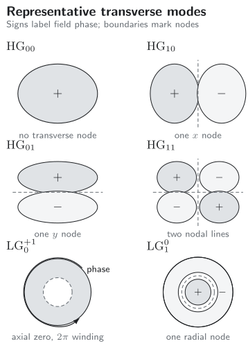

Representative scalar transverse modes at one plane. Gray lobes suggest intensity envelopes, while the $+$ and $-$ labels retain field phase information that an intensity image loses. $\mathrm{LG}_{0}^{+1}$ has an axial zero and one positive phase winding; $\mathrm{LG}_{1}^{0}$ has one radial node but no azimuthal winding.

The labels describe ideal basis functions. A measured pattern can be a coherent superposition, an incoherent spectral mixture, a clipped beam, or a distorted eigenmode. Visual resemblance is evidence, not a complete modal decomposition.

HG and LG Are Bases, Not Species

For one ideal isotropic paraxial system, all modes of total order

$$N = m+n = 2p+|\ell|$$

span the same $(N+1)$-dimensional degenerate subspace. HG and LG modes are different orthonormal bases for that subspace.

For example, first-order modes can be combined schematically as

$$u_{0,+1}^{\mathrm{LG}} \propto u_{10}^{\mathrm{HG}} + i u_{01}^{\mathrm{HG}},$$

and

$$u_{0,-1}^{\mathrm{LG}} \propto u_{10}^{\mathrm{HG}} - i u_{01}^{\mathrm{HG}}.$$

The relative phase of $\pm\pi/2$ turns two Cartesian lobed modes into a vortex mode. An astigmatic mode converter implements this transformation by giving the two axes different Gouy phases.

Geometry determines which basis is convenient:

Symmetry or perturbation	Natural description
rectangular aperture or astigmatism	HG-like modes
cylindrical symmetry	LG-like modes
elliptic coordinates	Ince–Gaussian modes
strong aperture or aberration	numerical round-trip modes
waveguide confinement	guided vector modes

Degeneracy means that any coherent superposition inside the subspace is also an eigenmode of the ideal symmetric problem. A small perturbation can select a different basis by diagonalizing the perturbation within that subspace.

Measuring a Mode

No single instrument measures every part of a laser-mode label.

Intensity images

A beam profiler measures a spatially sampled intensity,

$$I(x,y) \propto \left| \sum_\mu a_\mu u_\mu(x,y) \right|^2$$

if the fields remain mutually coherent during the exposure. Cross terms then depend on relative phase.

If frequency separations are large compared with the detector bandwidth, the exposure averages those terms:

$$\overline I(x,y) \simeq \sum_\mu |a_\mu|^2 |u_\mu(x,y)|^2.$$

The same camera image can therefore arise from a coherent superposition or an incoherent mixture. Background subtraction, finite sensor area, clipping, and saturation can further distort second moments and weak outer lobes.

Spectral measurements

A scanning Fabry–Pérot resonator or optical spectrum analyzer can resolve longitudinal frequencies if its resolution and free spectral range are appropriate. A fast photodetector can reveal intermode beat notes at

$$\nu_{\mathrm{beat}} = |\nu_\mu-\nu_\nu|.$$

Integrated detection can miss beats between orthogonal transverse modes because

$$\int u_\mu^*u_\nu\,dx\,dy = 0.$$

A local detector, aperture, or deliberate spatial projection prevents that orthogonality cancellation.

Phase-sensitive methods

Interferometry with a known reference reveals wavefront curvature, lobe signs, and phase singularities. Modal decomposition instead projects the complex field onto a chosen basis:

$$c_\mu = \int u_\mu^*(x,y) u(x,y) \,dx\,dy.$$

Intensity-only projections generally recover $|c_\mu|^2$, not all relative phases. Full reconstruction requires additional phase diversity, interferometry, wavefront sensing, or a tomographically complete set of measurements.

What “single mode” should report

A defensible report distinguishes:

Degree of freedom	Example evidence
longitudinal frequency	resolved optical spectrum or beat measurement
transverse field	phase-sensitive modal decomposition
polarization	Stokes parameters or polarization tomography
direction in a ring	separate clockwise and counterclockwise outputs
temporal state	coherence or photon-statistics measurement

A beam can be $\mathrm{HG}_{00}$ in space and still contain many longitudinal frequencies. It can be single-frequency but occupy two polarizations. It can also have $M^2$ near one while carrying technical phase and amplitude noise.

Beam Quality and M²

$M^2$ is a propagation measure, not a complete mode label. Define centered second moments in one transverse direction,

$$\begin{aligned} \sigma_x^2 &= \left\langle (x-\langle x\rangle)^2 \right\rangle, \\ \sigma_{\theta_x}^2 &= \left\langle (\theta_x-\langle\theta_x\rangle)^2 \right\rangle, \\ C_{x\theta} &= \left\langle (x-\langle x\rangle) (\theta_x-\langle\theta_x\rangle) \right\rangle. \end{aligned}$$

Then a scalar paraxial second-moment definition is

$$M_x^2 = \frac{4\pi}{\lambda} \sqrt{ \sigma_x^2\sigma_{\theta_x}^2 - C_{x\theta}^2 }.$$

The corresponding uncertainty inequality gives

$$M_x^2 \ge 1.$$

At a principal waist, an equivalent propagation law can be written

$$w_x^2(z) = w_{0x}^2 + \left[ \frac{M_x^2\lambda}{ \pi w_{0x} } \right]^2 (z-z_0)^2,$$

where $w_x=2\sigma_x$ is the second-moment radius.

For an ideal fundamental Gaussian, $M_x^2=M_y^2=1$. Larger values indicate a larger waist–divergence product, but do not uniquely identify the underlying mode mixture. Important limitations are:

• $M^2$ does not determine optical linewidth, polarization, or coherence;
• one transverse image cannot determine $M^2$;
• sensor noise at large radius can dominate a second moment;
• aperture clipping can make a measured beam appear deceptively narrow;
• strongly astigmatic beams need a full two-axis or four-dimensional moment treatment;
• a good $M^2$ fit does not prove that the field is an exact cavity eigenmode.

From Candidate Modes to Lasing Modes

Let $n_\mu$ be the photon number or a proportional modal intensity. A generic multimode rate equation is

$$\frac{dn_\mu}{dt} = \left[ G_\mu(\{n_\nu\}) - \kappa_\mu \right] n_\mu + S_\mu.$$

$G_\mu$ is saturated modal gain, $\kappa_\mu$ is modal loss, and $S_\mu$ represents spontaneous or other source terms. Near a stationary operating point, a useful expansion is

$$G_\mu-\kappa_\mu \simeq a_\mu - \sum_\nu b_{\mu\nu}n_\nu.$$

Here:

• $a_\mu$ is the unsaturated excess gain;
• $b_{\mu\mu}$ is self-saturation;
• $b_{\mu\nu}$ with $\mu\ne\nu$ is cross-saturation.

Ignoring source terms well above threshold gives

$$\frac{dn_\mu}{dt} = \left[ a_\mu - \sum_\nu b_{\mu\nu}n_\nu \right] n_\mu.$$

The first mode to cross threshold need not remain the only mode. Pump redistribution, thermal lensing, or weaker cross-saturation can let a second mode turn on later and suppress, coexist with, or destabilize the first.

The Two-Mode Competition Model

For two modes,

$$\begin{aligned} \dot n_1 &= \left( a_1 - b_{11}n_1 - b_{12}n_2 \right)n_1, \\ \dot n_2 &= \left( a_2 - b_{21}n_1 - b_{22}n_2 \right)n_2. \end{aligned}$$

Besides the off state and the two single-mode states, a coexistence solution has

$$\begin{aligned} n_1^* &= \frac{ a_1b_{22}-a_2b_{12} }{ D }, \\ n_2^* &= \frac{ a_2b_{11}-a_1b_{21} }{ D }, \\ D &= b_{11}b_{22} - b_{12}b_{21}. \end{aligned}$$

Physical coexistence requires both numerators and $D$ to give positive populations. A useful dimensionless coupling is

$$C = \frac{ b_{12}b_{21} }{ b_{11}b_{22} }.$$

For the symmetric case, $C<1$ permits stable coexistence: self-saturation is stronger than the combined cross-saturation. When $C>1$, the coexistence fixed point is unstable and one single-mode branch tends to exclude the other. Unequal excess gains decide which branch is reached; hysteresis or noise-driven switching can occur in suitable parameter ranges.

The model is local to a regime where mode shapes and saturation coefficients are fixed. It does not capture coherent population oscillations, beating near a material relaxation rate, four-wave mixing, or a mode basis that changes with pump.

What Sets Cross-Saturation?

Spatial overlap

For a local saturable gain medium, a schematic overlap is

$$b_{\mu\nu} \propto \int_{\mathrm{gain}} W(\mathbf r) |u_\mu(\mathbf r)|^2 |u_\nu(\mathbf r)|^2 \,d^3r,$$

where $W$ includes pump distribution, material density, and local saturation physics. Modes occupying different pumped regions interact weakly; modes sampling the same inversion interact strongly.

Homogeneous broadening

In a homogeneously broadened ensemble, each emitter contributes across the same line. Spectrally nearby modes then draw on nearly the same population, so cross-saturation can be comparable to self-saturation. This often favors a small number of oscillating frequencies.

Inhomogeneous broadening

In an inhomogeneously broadened ensemble, different frequency classes respond at different detunings. Two sufficiently separated modes can saturate partly distinct subensembles. Cross-saturation is then weaker and multifrequency oscillation is easier.

This contrast is not absolute. Velocity-changing collisions, spectral diffusion, population transport, power broadening, and coherent effects can reconnect nominally separate classes.

Spatial and spectral hole burning

Spatial hole burning is nonuniform depletion in position. Spectral hole burning is nonuniform depletion across an inhomogeneous frequency distribution. Both leave unsaturated resources that another mode can use. They should not be conflated:

• a standing-wave cavity can exhibit spatial holes even in a homogeneous line;
• a traveling-wave cavity can exhibit spectral holes in an inhomogeneous line;
• a real gain medium can exhibit both simultaneously.

Population transport

Diffusion, ballistic motion, carrier transport, and collisions refill holes. Fast transport makes the reservoir more nearly uniform and strengthens competition. Slow transport preserves local depletion and supports more independent modal reservoirs.

Practical Mode Selection

Mode selection works by changing excess gain $a_\mu$, saturation $b_{\mu\nu}$, or both.

Longitudinal selection

• Shorten the cavity so $\nu_{\mathrm{FSR}}$ exceeds the usable gain width.
• Add an etalon, grating, distributed reflector, or frequency-selective external cavity.
• Use a unidirectional ring to reduce standing-wave spatial hole burning.
• Seed the desired mode strongly enough to capture the available gain.
• Stabilize cavity length and gain-medium temperature to prevent hopping.

An intracavity filter does not merely “pick a frequency.” It changes loss, dispersion, group delay, and often spatial mode matching.

Transverse selection

• Match the pumped region to the desired fundamental mode.
• Use an aperture where higher-order modes have more intensity.
• Choose mirror curvature and cavity geometry with adequate mode discrimination.
• Reduce aberration, thermal lens asymmetry, and gain guiding.
• Couple into a single-mode waveguide or fiber when appropriate.

Apertures trade discrimination against diffraction loss and power handling. At high power, deliberately larger or higher-order modes can reduce intensity on optics; lowest order is not automatically optimal.

Polarization and direction

Birefringent elements, anisotropic gain, Brewster surfaces, wave plates, and polarizers split polarization modes. Faraday rotators or other nonreciprocal elements can favor one ring direction. Backscattering and polarization coupling must still be measured rather than assumed absent.

Worked Example: A Degenerate Spectrum

Consider an empty symmetric linear cavity with

$$L = 0.100\ \mathrm{m}, \qquad R_1=R_2 = 0.200\ \mathrm{m}.$$

Then

$$g_1=g_2 = 1-\frac{L}{R_i} = \frac12,$$

so

$$\alpha = \arccos \left( \frac12 \right) = \frac{\pi}{3}.$$

Using $c=2.99792458\times10^8\ \mathrm{m\,s^{-1}}$,

$$\nu_{\mathrm{FSR}} = \frac{c}{2L} \simeq 1.499\ \mathrm{GHz}.$$

One transverse-order step is

$$\Delta\nu_\perp = \frac13 \nu_{\mathrm{FSR}} \simeq 0.500\ \mathrm{GHz}.$$

The frequency factor for total order $N$ is

$$q+\frac{N+1}{3}.$$

Therefore

$$\nu_{q,N=3} = \nu_{q+1,N=0}.$$

The third-order transverse manifold is degenerate with the next longitudinal fundamental resonance in the ideal model. A small astigmatism splits the HG members; finite apertures give them different losses; pump overlap gives them different gains. The observed lasing spectrum is thus the perturbed active problem, not merely the ideal frequency table.

Common Mistakes

1. Calling every bright central spot TEM₀₀. A camera image lacks phase, and unresolved mixtures can look nearly Gaussian.
2. Using TEM without declaring the convention. In open optical resonators the fields are approximately transverse; exact vector modes can contain longitudinal components.
3. Confusing longitudinal and transverse single-mode operation. These are independent claims.
4. Treating $\mathrm{LG}_{+\ell}$ and $\mathrm{LG}_{-\ell}$ as distinguishable by intensity. Their ideal intensities are identical.
5. Equating a donut with orbital angular momentum. Phase winding, not annular intensity alone, establishes $\ell$.
6. Reading field signs from intensity lobes. Squaring removes the sign.
7. Using $M^2$ as a complete mode decomposition. It is one second-moment propagation metric.
8. Applying spherical-cavity formulas to a thermally distorted laser. The active mode and Gouy phase can depend on pump.
9. Assuming the lowest-loss mode always wins far above threshold. Nonlinear cross-saturation and mode reshaping can reorder the branches.
10. Calling all holes spatial hole burning. Frequency-selective depletion is spectral hole burning.

Mode-Analysis Workflow

For an unfamiliar laser:

1. Specify whether the question concerns frequency, transverse field, polarization, direction, or temporal statistics.
2. Compute or measure passive resonances and losses before adding gain.
3. Choose a basis matched to the actual symmetry and waist.
4. Record transverse profiles at several axial planes with calibrated background and sensor area.
5. Resolve optical frequencies or beat notes on the relevant bandwidth.
6. Add phase-sensitive or projective measurements if modal coefficients are required.
7. Vary pump and alignment to distinguish a fixed passive mode from an active, pump-dependent mode.
8. Fit a multimode saturation model only after checking whether its mode shapes remain approximately fixed.

The result should state both the inferred mode content and the evidence that rules out plausible alternatives.

Exercises

1. Normalize the fundamental Gaussian

At a fixed plane, let

$$u_{00}(r) = A \exp \left( -\frac{r^2}{w^2} \right).$$

Find $A>0$ from

$$\int_{\mathbb R^2} |u_{00}|^2\,d^2r = 1.$$

Verify that $r=w$ is the $e^{-2}$ intensity radius.

Solution

Using polar coordinates,

$$\begin{aligned} 1 &= 2\pi A^2 \int_0^\infty r \exp \left( -\frac{2r^2}{w^2} \right) dr \\ &= 2\pi A^2 \frac{w^2}{4}. \end{aligned}$$

Therefore

$$A = \sqrt{\frac{2}{\pi}} \frac{1}{w}.$$

The intensity ratio is

$$\frac{I(r)}{I(0)} = \exp \left( -\frac{2r^2}{w^2} \right).$$

At $r=w$ this equals $e^{-2}$. The rms radius and diameter are different quantities.

2. Read an HG mode from its indices

For the ideal mode $\mathrm{HG}_{20}$:

1. find its total transverse order;
2. locate its nodal lines at the waist;
3. state its parity under $x\mapsto-x$ and $y\mapsto-y$;
4. find $M_x^2$ and $M_y^2$.

Use $H_2(\xi)=4\xi^2-2$.

Solution

The total order is

$$N = m+n = 2.$$

The Hermite argument is

$$\xi = \frac{\sqrt2\,x}{w_0}.$$

$H_2(\xi)=0$ at $\xi=\pm1/\sqrt2$, so the vertical nodal lines are

$$x = \pm\frac{w_0}{2}.$$

There is no horizontal nodal line because $n=0$. $H_2$ is even and $H_0=1$, so the field is even under both reflections. Finally,

$$M_x^2 = 2m+1 = 5, \qquad M_y^2 = 2n+1 = 1.$$

The mode is diffraction-limited in the $y$ direction but not in the $x$ direction.

3. Distinguish LG intensity from phase

Consider $\mathrm{LG}_{1}^{-2}$.

1. How many radial nodes does it have?
2. What happens to its intensity on the axis?
3. What is its total transverse order?
4. What is its paraxial axial orbital angular momentum per photon?
5. Can an ideal intensity image distinguish it from $\mathrm{LG}_{1}^{+2}$?

Solution

$p=1$ gives one radial node. Because $|\ell|=2$, the amplitude contains $r^2$ and vanishes quadratically on the axis; the intensity vanishes as $r^4$.

The total order and beam quality are

$$N = 2p+|\ell| = 4,$$

and

$$M^2 = N+1 = 5.$$

The azimuthal factor is $e^{-2i\phi}$, so

$$L_z = -2\hbar$$

per photon in the scalar paraxial description. Changing $\ell$ from $-2$ to $+2$ complex-conjugates the azimuthal phase but leaves $|u|^2$ unchanged. An ideal intensity image cannot determine the sign. Interference or another phase-sensitive measurement is required.

4. Find a cavity degeneracy

For the symmetric cavity in the worked example,

$$\alpha = \frac{\pi}{3}.$$

Show that every increase of three in total transverse order can be offset by one longitudinal free spectral range. Give one HG mode of order three that is degenerate with a neighboring fundamental mode.

Solution

The dimensionless resonance factor is

$$q+\frac{N+1}{3}.$$

Increasing $N$ by three adds one:

$$q+\frac{N+4}{3} = (q+1)+\frac{N+1}{3}.$$

For $N=0$ and $N=3$,

$$\nu_{q,3} = \nu_{q+1,0}.$$

The order-three HG modes are

$$\mathrm{HG}_{30}, \quad \mathrm{HG}_{21}, \quad \mathrm{HG}_{12}, \quad \mathrm{HG}_{03}.$$

Thus, for example, $\mathrm{HG}_{30}$ with longitudinal index $q$ is degenerate with $\mathrm{HG}_{00}$ at $q+1$ in the ideal cavity. Apertures, astigmatism, gain overlap, and aberration generally split their thresholds even when their ideal frequencies coincide.

5. Compute an astigmatic splitting

An astigmatic cavity has

$$\alpha_x = \frac{\pi}{3}, \qquad \alpha_y = \frac{\pi}{4}, \qquad \nu_{\mathrm{FSR}} = 1.50\ \mathrm{GHz}.$$

Find $\nu_{q10}-\nu_{q01}$.

Solution

Using the axis-resolved spectrum,

$$\begin{aligned} \nu_{q10}-\nu_{q01} &= \frac{\alpha_x-\alpha_y}{\pi} \nu_{\mathrm{FSR}} \\ &= \left( \frac13-\frac14 \right) (1.50\ \mathrm{GHz}) \\ &= 0.125\ \mathrm{GHz}. \end{aligned}$$

Therefore

$$\nu_{q10}-\nu_{q01} = 125\ \mathrm{MHz}.$$

The sign says that the $x$-excited mode lies higher for the stated branch convention.

6. Analyze symmetric two-mode competition

Take

$$a_1=a_2=a>0, \qquad b_{11}=b_{22}=b>0, \qquad b_{12}=b_{21}=cb.$$

Find the coexistence fixed point and determine its linear stability for $c<1$ and $c>1$.

Solution

Symmetry gives

$$n_1^* = n_2^* = n^*.$$

The zero-growth condition is

$$a-bn^*-cbn^* = 0,$$

so

$$n^* = \frac{a}{b(1+c)}.$$

At this point, the Jacobian is

$$J = -bn^* \begin{pmatrix} 1 & c\\ c & 1 \end{pmatrix}.$$

Its symmetric and antisymmetric eigenvalues are

$$\lambda_+ = -a,$$

and

$$\lambda_- = -a \frac{1-c}{1+c}.$$

The symmetric perturbation always decays. If $c<1$, the antisymmetric perturbation also decays and coexistence is stable. If $c>1$, the antisymmetric perturbation grows: one mode rises while the other falls.

The single-mode state $(a/b,0)$ gives the absent second mode a small-signal growth rate

$$a-cb\frac{a}{b} = a(1-c).$$

It is stable against invasion when $c>1$. The equivalent statement holds for the other single-mode branch.

7. Quantify standing-wave spatial hole burning

Define normalized longitudinal intensity patterns on $0<z<L$ by

$$f_q(z) = 2 \sin^2 \left( \frac{q\pi z}{L} \right),$$

so that their spatial average is one. Compute the self-overlap

$$\left\langle f_q^2 \right\rangle$$

and the cross-overlap

$$\left\langle f_qf_r \right\rangle$$

for distinct positive integers $q\ne r$. Compare the cross-overlap with the self-overlap.

Solution

Using

$$\left\langle \sin^4 \right\rangle = \frac38,$$

the self-overlap is

$$\left\langle f_q^2 \right\rangle = 4 \left\langle \sin^4 \right\rangle = \frac32.$$

For distinct integer harmonics, all oscillatory cross terms average to zero:

$$\left\langle \sin^2 \left( \frac{q\pi z}{L} \right) \sin^2 \left( \frac{r\pi z}{L} \right) \right\rangle = \frac14.$$

Hence

$$\left\langle f_qf_r \right\rangle = 1.$$

Relative to self-saturation, the cross-saturation from this ideal longitudinal overlap is

$$\frac{ \langle f_qf_r\rangle }{ \langle f_q^2\rangle } = \frac23.$$

Different standing waves therefore compete less strongly than a mode competes with itself. In an ideal uniform traveling wave, $f=1$ and both self- and cross-overlaps equal one. This calculation isolates the spatial effect; spectral and transverse overlaps can change the full coefficient.

8. Decide when a beat note survives detection

Two fields are

$$\mathcal E = a_1u_1(x,y)e^{-i\omega_1t} + a_2u_2(x,y)e^{-i\omega_2t}.$$

Derive the interference term in the intensity. Explain when it disappears because of detector bandwidth and when it disappears because of spatial integration.

Solution

The intensity contains

$$\begin{aligned} I(x,y,t) \propto& |a_1|^2|u_1|^2 + |a_2|^2|u_2|^2 \\ &+ 2\operatorname{Re} \left[ a_1a_2^* u_1u_2^* e^{-i(\omega_1-\omega_2)t} \right]. \end{aligned}$$

The last line oscillates at

$$\Omega = |\omega_1-\omega_2|.$$

A detector whose integration time is much longer than $2\pi/\Omega$ averages that term to zero. A sufficiently fast local detector can retain it.

Even a fast detector that integrates the complete transverse plane gives a cross term proportional to

$$\int u_1u_2^* \,dx\,dy.$$

This vanishes for exactly orthogonal modes. A finite aperture, local detector, deliberate mode projection, or imperfect orthogonality can restore the beat. Detector bandwidth and spatial orthogonality are therefore independent reasons for a missing signal.

References

1. A. E. Siegman, Lasers, University Science Books (1986). A standard treatment of Gaussian beams, resonator modes, apertures, mode selection, and laser oscillation.
2. H. Kogelnik and T. Li, “Laser Beams and Resonators,” Applied Optics 5, 1550–1567 (1966). The classic unified review of paraxial beams and optical resonators.
3. A. G. Fox and T. Li, “Resonant Modes in a Maser Interferometer,” Bell System Technical Journal 40, 453–488 (1961). The foundational numerical round-trip treatment of finite-aperture resonator modes.
4. A. E. Siegman, “Hermite–Gaussian Functions of Complex Argument as Optical-Beam Eigenfunctions,” Journal of the Optical Society of America 63, 1093–1094 (1973).
5. J. Enderlein and F. Pampaloni, “Unified Operator Approach for Deriving Hermite–Gaussian and Laguerre–Gaussian Laser Modes,” Journal of the Optical Society of America A 21, 1553–1558 (2004).
6. L. Allen, M. W. Beijersbergen, R. J. C. Spreeuw, and J. P. Woerdman, “Orbital Angular Momentum of Light and the Transformation of Laguerre–Gaussian Laser Modes,” Physical Review A 45, 8185–8189 (1992).
7. A. E. Siegman, “Defining, Measuring, and Optimizing Laser Beam Quality,” Proceedings of SPIE 1868, 2–12 (1993).
8. W. E. Lamb, Jr., “Theory of an Optical Maser,” Physical Review 134, A1429–A1450 (1964). A foundational semiclassical theory of frequency selection, saturation, and multimode interaction.
9. C. L. Tang, H. Statz, and G. deMars, “Spectral Output and Spiking Behavior of Solid-State Lasers,” Journal of Applied Physics 34, 2289–2295 (1963). An early quantitative treatment of multimode dynamics and spatial hole burning.
10. W. R. Bennett, Jr., “Hole Burning Effects in a He–Ne Optical Maser,” Physical Review 126, 580–593 (1962).
11. O. Svelto, Principles of Lasers, 5th ed., Springer (2010). A graduate-level account of resonators, transverse modes, gain saturation, and mode selection.
12. H. Haken, Laser Theory, Springer (1984). A systematic treatment of multimode laser dynamics, competition, and instability.
13. M. Sargent III, M. O. Scully, and W. E. Lamb, Jr., Laser Physics, Addison-Wesley (1974). A detailed semiclassical treatment of homogeneous and inhomogeneous broadening and mode interaction.
14. P. W. Milonni and J. H. Eberly, Laser Physics, Wiley (2010). A modern bridge from Maxwell–Bloch dynamics to practical laser behavior.