Frequency Standards

A frequency standard is a measurement standard whose assigned quantity value is a frequency. In an atomic implementation, a quantum transition supplies a reproducible reference, an oscillator supplies continuous phase, an interrogation and feedback system connects the two, and synthesis or a frequency comb makes a usable output. The result is not merely a narrow spectral line. It is a specified frequency at a specified reference plane, with a correction model, an uncertainty, a stability characterization, and a documented route to a reference such as the SI second.

The distinction matters because different parts of the instrument answer different questions:

• the reference determines what frequency should be realized;
• the oscillator carries phase between observations of the reference;
• the servo estimates and corrects their frequency difference;
• the synthesis chain maps the disciplined oscillator to an output;
• the comparison link connects that output to another standard;
• the traceability record states what reference was used, when it was used, and what uncertainty every link contributed.

A standard can have excellent short-term stability but an incorrect assigned value. It can have a small systematic uncertainty but poor availability. It can be traceable yet unsuitable for a demanding application because its uncertainty is too large. These are separate properties, not synonyms.

Canonical Scope

This page owns the realization, comparison, and traceability architecture of frequency standards:

1. the operational distinctions among oscillator, reference, frequency standard, clock, flywheel, and time scale;
2. the chain from a transition to a defined microwave or optical output;
3. frequency comparison through phase, counters, synthesis, and optical ratios;
4. the use and limits of Allan deviation and related stability statistics;
5. primary frequency standards, secondary frequency standards, and secondary representations of the second;
6. metrological traceability, calibration intervals, dead time, and holdover;
7. the roles of UTC($k$), EAL, TAI, UTC, UTCr, Circular T, CCTF-K001.UTC, and TT(BIPM);
8. frequency transfer by GNSS, two-way satellite methods, optical fiber, and other links; and
9. the evidence needed for a reproducible, traceable frequency result.

Neighboring pages retain their canonical roles:

• Atomic Clocks owns clock transitions, passive clock cycles, microwave architectures, projection noise, local-oscillator aliasing, and the Dick effect.
• Optical Clocks owns trapped-ion and lattice implementations, optical-clock systematics, relativistic geodesy, and optical-clock tests of fundamental physics.
• Frequency Combs derives comb-tooth frequencies, self-referencing, transfer oscillators, and optical frequency division.
• Laser Stabilization owns discriminator noise, feedback transfer functions, loop stability, reference cavities, and out-of-loop verification.
• Precision Spectroscopy owns line-center inference and detailed spectroscopic uncertainty evaluation.
• Precision Measurement and Metrology owns the general vocabulary of measurands, covariance propagation, uncertainty, and validation shared by all AMO sensors.

The purpose here is therefore not to repeat a clock servo or comb derivation. It is to show how those components become a metrological standard and how a comparison becomes a defensible calibration.

The Objects in a Frequency Laboratory

Oscillator

An oscillator produces a signal with evolving phase. Write a nominal sinusoidal output as

$$V(t) = V_0\cos\!\left[ 2\pi\nu_{\rm nom}t+\phi(t) \right].$$

The instantaneous frequency is

$$\nu(t) = \nu_{\rm nom} + \frac{1}{2\pi}\frac{d\phi}{dt}.$$

Quartz oscillators, dielectric resonators, lasers, cryogenic resonators, and hydrogen masers can all serve as oscillators. An oscillator need not possess an accurate absolute frequency. Its central metrological asset is continuous phase with sufficiently predictable fluctuations over the interval between calibrations.

Reference

A frequency reference provides a reproducible condition that identifies a frequency. An atomic transition, an optical cavity mode, a molecular spectral line, or a signal received from another laboratory can act as a reference. A reference need not itself supply a continuous output.

An unperturbed transition frequency

$$\nu_0 = \frac{E_e-E_g}{h}$$

is a theoretical and operational specification. The laboratory observes a perturbed resonance, estimates shifts, and connects an oscillator to the specified unperturbed value. “The atom has frequency $\nu_0$” is shorthand for this measurement model, not a complete description of the apparatus.

Frequency standard

A frequency standard realizes, conserves, or reproduces an assigned frequency value. The term may refer to:

• a primary or secondary atomic standard evaluated against the SI second;
• a continuously operating reference oscillator with a calibration;
• a working standard used to calibrate laboratory instruments;
• a travelling standard transported between laboratories; or
• a remote reference delivered through a calibrated transfer link.

The standard includes the relevant output plane and measurement procedure. Two nominally identical $10\ \mathrm{MHz}$ ports are not interchangeable if their distribution amplifiers, cables, or synthesizers contribute different offsets, phase steps, or noise.

Clock

A clock combines a frequency source with a procedure for assigning time or phase. If $C(t)$ is its reading and $t$ is a reference coordinate time, the time error is

$$x(t) = C(t)-t.$$

Frequency is the rate of clock time. A standard can provide frequency without publishing an epoch, while a clock must maintain both rate and a time reading. Conversely, a clock display can appear synchronized even if its oscillator has poor free-running frequency because it is corrected frequently.

Flywheel and holdover oscillator

A flywheel bridges intervals when a more accurate reference is unavailable. Hydrogen masers often serve this role between intermittent optical-clock evaluations. A flywheel is selected for predictable phase and frequency evolution over the relevant gap, not merely for the smallest one-second Allan deviation.

Holdover is operation without the external calibration input. The resulting uncertainty depends on the prior estimate of offset and drift, the oscillator noise model, the duration of the outage, and any environmental sensitivity. It is a prediction problem.

Time scale

A time scale is an algorithmic and operational procedure that combines clock data into a reference time. A schematic ensemble is

$$x_{\rm ens}(t) = \sum_{i=1}^{N} w_i \left[ x_i(t)+p_i(t) \right], \qquad \sum_{i=1}^{N}w_i=1,$$

where $x_i$ is a measured clock difference and $p_i$ is a prediction or steering term. Real algorithms estimate clock rates, drift, outliers, and future behavior; they also limit individual weights and preserve continuity. The computed ensemble must ultimately be represented by physical outputs.

The algorithm can be more stable than any typical member while remaining dependent on external standards for its long-term rate. An ensemble, a primary standard, and a disseminated time signal are therefore different objects.

A compact vocabulary table

Object	What it supplies	Typical weakness	Example
oscillator	continuous phase	unknown or drifting absolute frequency	quartz oscillator, laser
reference	reproducible frequency condition	may be intermittent or noncontinuous	atomic transition, cavity
standard	assigned frequency with procedure and uncertainty	limited uptime, calibration, or transfer	caesium fountain, calibrated maser
flywheel	predictable phase between calibrations	accumulates prediction error	hydrogen maser
clock	frequency plus epoch or time reading	steering can cause phase or rate artifacts	UTC($k$) output
time scale	computed ensemble time	depends on data latency and steering policy	EAL, TAI, UTC
transfer link	comparison between locations	delay variation and calibration	GNSS, TWSTFT, optical fiber

Convention Ledger

Frequency metrology is unusually sensitive to sign, epoch, and reference plane. This page uses the following conventions.

Phase time and fractional frequency

Let $\phi(t)$ be the phase deviation of a signal from a nominal oscillator at frequency $\nu_{\rm nom}$. Its phase-time deviation is

$$x(t) = \frac{\phi(t)}{2\pi\nu_{\rm nom}}.$$

Its fractional-frequency deviation is

$$y(t) = \frac{\nu(t)-\nu_{\rm nom}}{\nu_{\rm nom}} = \frac{dx}{dt}.$$

The interval-average fractional frequency from $t_1$ to $t_2$ is

$$\overline{y}_{[t_1,t_2]} = \frac{x(t_2)-x(t_1)}{t_2-t_1}.$$

This endpoint relation is exact for the interval average under the stated definition. It is also why a phase record is often more informative than a list of already averaged frequency values: phase steps, gaps, and time-tag errors remain visible.

For two clocks $A$ and $B$, define

$$x_{A-B}(t)=x_A(t)-x_B(t), \qquad y_{A-B}(t)=y_A(t)-y_B(t).$$

A report must state its sign convention explicitly. BIPM products use expressions such as $[\mathrm{UTC}-\mathrm{UTC}(k)]$; silently reversing that sign reverses the inferred correction.

Frequency and angular frequency

Ordinary frequency is denoted $\nu$ or $f$ and measured in hertz. Angular frequency is $\omega=2\pi\nu$. Mixing them introduces a factor of $2\pi$ in phase, linewidth, and servo calculations.

Reference planes

Every output is defined at a physical or logical reference plane:

• a connector on a distribution amplifier;
• an optical plane before or after an acousto-optic modulator;
• the input of a counter;
• the effective antenna phase center of a transfer receiver; or
• a software epoch after a documented delay correction.

If a cable of delay $d(t)$ lies between the defined plane and the counter, the measured phase time includes that delay. A changing delay causes a fractional-frequency bias

$$y_{\rm delay}(t) = \frac{dd}{dt}.$$

A constant delay affects time synchronization but not a long-term frequency average; a changing delay affects both. This distinction is central to frequency transfer.

Coordinate and proper frequency

Atomic standards operate along physical worldlines and realize proper-time rates. International comparisons refer them to specified coordinate-time conventions and gravitational reference potentials. To first order in a weak stationary field,

$$\frac{\Delta\nu}{\nu} \simeq \frac{\Delta U}{c^2},$$

where the sign follows the stated potential convention. The gravitational correction and its uncertainty belong in a primary or secondary standard’s evaluation. A location label alone is not an adequate potential model.

From a Transition to a Usable Standard

The physical chain

The minimal passive atomic chain is

$$\text{oscillator} \longrightarrow \text{atoms} \longrightarrow \text{discriminator} \longrightarrow \text{servo} \longrightarrow \text{oscillator}.$$

The atoms are observed intermittently or continuously, and the discriminator estimates an error proportional to the detuning near its operating point. The servo steers one or more oscillator actuators. A synthesis chain then produces the frequency needed by users or comparisons.

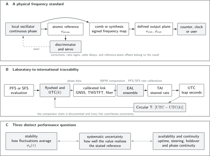
A frequency standard is both a physical signal chain and a documented comparison chain. Panel A separates the atomic reference from the continuous oscillator and defines the output plane. Panel B shows one route from a primary or secondary frequency standard through UTC($k$) and calibrated links to BIPM time-scale products. The arrows do not imply that UTC is generated in real time from a single standard: EAL, TAI, and UTC are computed from submitted data, while laboratories maintain real-time local realizations. Panel C emphasizes that stability, systematic uncertainty, and availability answer different questions.

Locking to a transition

Suppose an interrogation produces an observable $P(\delta)$ as a function of detuning

$$\delta = 2\pi(\nu_{\rm LO}-\nu_{\rm atom}).$$

Sampling on opposite sides of the resonance gives a signed error signal, for example

$$e_k = P_k(+\Delta)-P_k(-\Delta) \simeq K_d\,\delta_k+b_k,$$

where $K_d$ is the discriminator slope and $b_k$ collects offsets and asymmetries. A discrete controller updates an oscillator command:

$$u_{k+1} = u_k-g e_k -g_I\sum_{j\le k}e_j.$$

The sign of $gK_d$ must provide negative feedback. The loop bandwidth must be high enough to suppress useful oscillator noise but low enough to remain stable despite interrogation delay, sampling, and actuator dynamics.

This concise model hides the clock-specific physics. Ramsey phases, line shapes, projection noise, dead time, and the Dick effect are developed in Atomic Clocks and Ramsey Interferometry. Generic feedback design is developed in Laser Stabilization.

The realized frequency

The servo lock point is not automatically the unperturbed transition. A generic realization model is

$$\nu_{\rm std} = \nu_{\rm out} -\sum_i \Delta\nu_i -\Delta\nu_{\rm synth} -\Delta\nu_{\rm link},$$

or, in fractional form,

$$y_{\rm std} = y_{\rm out} -\sum_i c_i -c_{\rm synth} -c_{\rm link}.$$

Here $\Delta\nu_i$ are physical shifts of the reference, while synthesis and link terms move the measured output relative to the defined plane. A correction is an estimate with uncertainty, not a declaration that the effect has vanished.

For input quantities $q_i$, a local linearized model gives

$$\Delta\nu_i \simeq k_i(q_i-q_{i,0}),$$

and the combined variance includes covariance:

$$u^2(\nu_{\rm std}) = \sum_{i,j} \frac{\partial\nu_{\rm std}}{\partial q_i} \frac{\partial\nu_{\rm std}}{\partial q_j} \operatorname{cov}(q_i,q_j).$$

The detailed physical ledgers for microwave and optical standards belong to the clock pages. The metrological point is that the assigned output value must include the correction model valid during the stated evaluation interval.

Active and passive standards

In a passive standard, an external oscillator interrogates a transition and is steered by the response. In an active standard, stimulated emission or masing produces the output field directly. A hydrogen maser is the canonical active example.

“Active” does not mean free of calibration. Cavity pulling, state preparation, magnetic fields, wall interactions, and aging still affect the output. Active standards are often excellent flywheels, while passive primary standards can provide superior long-term accuracy.

Synthesis and division

A user rarely receives the transition frequency directly. Microwave standards use multipliers, dividers, phase-locked loops, and direct digital synthesis. Optical standards use a comb to connect hundreds of terahertz to radio frequency or to another optical carrier.

For a continuous-wave optical frequency measured against a comb,

$$\nu_{\rm cw} = n f_{\rm rep} +f_{\rm CEO} +s_b f_b +\sum_j s_j f_{{\rm AOM},j},$$

where $n$ is the tooth index and the signs $s_b,s_j=\pm1$ are determined from the optical layout and actuator conventions. The canonical derivation, self-referencing conditions, and transfer-oscillator combinations are in Frequency Combs.

The synthesis uncertainty is not necessarily limited by nominal electronic resolution. Cycle slips, wrong tooth indices, untracked phase-lock offsets, counter dead time, distribution noise, and sign errors can dominate. A metrological implementation records every term and verifies the result out of loop.

Output phase continuity

A frequency correction can be applied in two qualitatively different ways:

1. a phase step changes the clock reading immediately;
2. a frequency steering changes the slope of phase and removes the offset gradually.

If phase continuity matters, a synthesizer update should preserve phase or the phase step must be measured and documented. A frequency standard used only for interval calibration may tolerate a known phase step; a time scale or coherent network often cannot.

Comparing Frequencies

Comparison is the observable

No instrument measures an isolated absolute frequency. It measures a phase or frequency difference, ratio, or beat against another oscillator. The basic comparison result is

$$y_{A-B} = \frac{\nu_A-\nu_B}{\nu_0},$$

with a clearly defined normalization $\nu_0$. For very different carrier frequencies, a ratio is more natural:

$$R_{AB} = \frac{\nu_A}{\nu_B}.$$

An absolute frequency measurement means a comparison whose chain ends at a realization of the SI second. It does not mean a measurement without a reference. An optical ratio can be much more precise than either optical frequency’s absolute calibration because it avoids a microwave link and several common uncertainty terms.

Phase endpoints and mean frequency

If a comparison system records $x_{A-B}(t)$, the interval-average fractional-frequency difference is

$$\overline{y}_{A-B} = \frac{x_{A-B}(t_2)-x_{A-B}(t_1)} {t_2-t_1}.$$

For a complete, continuous record this endpoint estimator is insensitive to bounded phase noise in the long-average limit. In practice, gaps, outliers, phase wraps, and changing delays require a documented estimator. A linear fit can use all samples, but its weighting and response to nonstationary noise must be stated.

A phase step $\Delta x$ inside an interval of duration $T$ biases a simple endpoint frequency estimate by

$$\Delta\overline{y} = \frac{\Delta x}{T}.$$

Thus a $1\ \mathrm{ns}$ unrecorded step biases a one-day average by about $1.16\times10^{-14}$. Small timing discontinuities are not small at the fractional-frequency levels of modern standards.

Frequency counters

A counter estimates phase change over a gate. An ideal rectangular, dead-time-free average is

$$\overline{\nu}_k = \frac{\phi(t_k+\tau)-\phi(t_k)} {2\pi\tau}.$$

Real counters can use different estimators and weighting functions. Common categories include:

• rectangular or $\Pi$-type averaging;
• triangular or $\Lambda$-type averaging from overlapped estimates;
• regression-based frequency estimates; and
• timestamp or phase-recorder outputs.

Two data streams labelled “one-second frequency” need not have the same transfer function. Counter mode affects white-phase-noise rejection, adjacent-sample correlations, and which Allan statistic is appropriate. A report should state the instrument, mode, gate time, dead time, input bandwidth, trigger level, and common timebase.

Common timebases and false agreement

If two counters share a timebase derived from one of the standards, the result can contain useful common-mode rejection, but it can also hide errors. A ratio counter that references both channels to the same oscillator does not independently validate that oscillator. Likewise, two nominally independent comb paths can share an RF reference, fiber, synthesizer, or software sign convention.

An out-of-loop comparison should be independent in the mechanism relevant to the claim. Independence is architectural, not merely a second line on a plot.

Optical ratios and closure

For standards $A$, $B$, and $C$, a ratio network should satisfy

$$R_{AB}R_{BC}R_{CA}=1.$$

Define a logarithmic closure residual

$$\epsilon_{\rm cl} = \ln R_{AB}+\ln R_{BC}+\ln R_{CA}.$$

For small errors, $\epsilon_{\rm cl}$ is approximately the sum of fractional ratio errors. A nonzero residual reveals inconsistency but does not by itself identify which standard, comb, or link is wrong. Shared errors can also cancel around the loop, so closure is powerful evidence, not a proof that every component is correct.

Absolute frequency through a flywheel

An intermittent optical standard can calibrate a continuous maser, which is then compared with UTC($k$) or TAI. A schematic decomposition is

$$y_{\rm opt-SI} = y_{\rm opt-H} +y_{\rm H-UTC(k)} +y_{\rm UTC(k)-TAI} +y_{\rm TAI-SI}.$$

Every term must refer to compatible intervals and sign conventions. Interpolating or extrapolating the maser over optical-clock dead time adds uncertainty that depends on the maser’s noise process and the placement of the measurement epochs. Equal uptime fractions can produce different dead-time uncertainties if the gaps are distributed differently.

Stability Statistics

Why ordinary variance is often unsuitable

Clock noise commonly includes flicker frequency noise, random-walk frequency noise, and drift. The classical variance of frequency samples can depend strongly on record length and need not converge for these processes. Frequency metrology therefore uses differenced statistics that are finite for important power-law noise classes and explicitly depend on averaging time $\tau$.

Stability is a property of a process and measurement bandwidth. A single number without $\tau$, estimator, data treatment, and confidence information is incomplete.

Allan variance

For contiguous interval averages $\overline y_k(\tau)$, the two-sample Allan variance is

$$\sigma_y^2(\tau) = \frac{1}{2} \left\langle \left[ \overline y_{k+1}(\tau) -\overline y_k(\tau) \right]^2 \right\rangle.$$

In terms of phase-time samples $x_k=x(t_0+k\tau)$,

$$\sigma_y^2(\tau) = \frac{1}{2\tau^2} \left\langle \left( x_{k+2}-2x_{k+1}+x_k \right)^2 \right\rangle.$$

The Allan deviation is $\sigma_y(\tau)$. It characterizes fluctuation amplitude after averaging for time $\tau$; it is not the systematic uncertainty of the standard.

For a finite record with $M$ nonoverlapping frequency averages,

$$\widehat{\sigma}_y^2(\tau) = \frac{1}{2(M-1)} \sum_{k=0}^{M-2} \left( \overline y_{k+1}-\overline y_k \right)^2.$$

Overlapping estimators reuse the phase data to improve statistical confidence, especially at long $\tau$. The terms are then correlated, so the number of plotted points is not the number of independent degrees of freedom.

Reading slopes

For ideal power-law noises, log–log Allan-deviation slopes provide a useful diagnostic:

Dominant noise	Typical phase/frequency description	Allan-deviation scaling
white phase modulation	independent fast phase measurement noise	approximately $\tau^{-1}$, bandwidth dependent
flicker phase modulation	$1/f$ phase noise	approximately $\tau^{-1}$ with logarithmic/bandwidth dependence
white frequency modulation	independent frequency averages	$\tau^{-1/2}$
flicker frequency modulation	$1/f$ frequency noise	$\tau^0$
random-walk frequency modulation	integrated white frequency increments	$\tau^{+1/2}$
deterministic linear frequency drift	predictable slope in $y(t)$	$\tau^{+1}$ if not removed

These are model signatures, not automatic identifications. Mixed noise, filtering, periodic environmental modulation, data gaps, and servo features can mimic slopes over a limited range.

Modified Allan deviation

Modified Allan variance adds averaging before the two-sample difference. It is especially useful for distinguishing white from flicker phase modulation, which ordinary Allan deviation does not reliably separate by slope. Its value depends on the base sampling interval and estimator definition.

For phase samples separated by $\tau_0$ and $\tau=m\tau_0$, one common overlapping form is

$$\operatorname{mod}\sigma_y^2(\tau) = \frac{1}{2m^2\tau^2} \left\langle \left[ \sum_{i=0}^{m-1} \left( x_{k+2m+i}-2x_{k+m+i}+x_{k+i} \right) \right]^2 \right\rangle.$$

Software packages differ in accepted input type, overlap convention, and normalization. A publication should name the implementation or state the formula.

Hadamard deviation

Hadamard variance uses a second difference of interval-average frequency, equivalently a third difference of phase:

$$\sigma_H^2(\tau) = \frac{1}{6} \left\langle \left( \overline y_{k+2} -2\overline y_{k+1} +\overline y_k \right)^2 \right\rangle.$$

It is insensitive to linear frequency drift. That makes it useful for characterizing clocks whose drift is substantial or difficult to remove without introducing analyst choices. It does not make drift irrelevant to prediction or holdover.

Time deviation

Time deviation, TDEV, expresses the dispersion of timing error rather than fractional frequency. Under the standard modified-Allan convention,

$$\operatorname{TDEV}(\tau) = \frac{\tau}{\sqrt{3}}\, \operatorname{mod}\sigma_y(\tau).$$

This relation is convention dependent through the definition of modified Allan deviation. TDEV is useful for synchronization and time-transfer applications, while Allan deviation is usually more direct for frequency standards.

Stability does not equal uncertainty of a mean

It is tempting to infer

$$u_A(\overline y) \stackrel{?}{=} \frac{\sigma_y(\tau_0)}{\sqrt{T/\tau_0}}.$$

That relation is valid only under assumptions close to independent white frequency noise. Flicker floors, random walk, drift, dead time, correlations, and estimator filtering change the uncertainty of the average. A defensible Type A evaluation uses the observed noise model, the actual sampling pattern, and sensitivity to analysis choices.

Three-cornered comparisons

A beat between $A$ and $B$ measures the sum of their noise contributions and any link noise. If three standards are mutually compared and their noises are uncorrelated, one may estimate

$$\sigma_A^2 = \frac{1}{2} \left( \sigma_{AB}^2 +\sigma_{AC}^2 -\sigma_{BC}^2 \right),$$

with cyclic expressions for $B$ and $C$. Correlations, common reference noise, shared links, or estimator differences invalidate the simple decomposition and can even produce negative variance estimates. A three-cornered hat is a model-based inference, not a direct single-clock measurement.

Dead time and gaps

Dead time changes the statistical question. For white frequency noise, separated samples merely reduce the effective sample count. For flicker or random-walk frequency noise, unobserved evolution during gaps can dominate. The uncertainty depends on:

• noise type and fitted coefficients;
• gap lengths and locations;
• interpolation or extrapolation algorithm;
• calibration interval and endpoint constraints;
• whether a continuously observed flywheel bridges the gaps; and
• correlations between the flywheel and the comparison link.

Monte Carlo simulation from a validated noise model is often appropriate, but its result is only as trustworthy as the model, parameter estimates, and gap pattern supplied to it.

Primary, Secondary, and Working Standards

The SI second in 2026

As reviewed on 25 July 2026, the SI second remains defined by fixing the unperturbed ground-state hyperfine transition frequency of the caesium-133 atom:

$$\Delta\nu_{\rm Cs} = 9\,192\,631\,770\ \mathrm{Hz}.$$

The definition refers to an unperturbed atom, and its practical realization requires corrections for environmental, motional, and relativistic effects. Optical standards can realize secondary representations with uncertainties below those of the best caesium fountains, but this does not make an optical transition the present defining transition.

Primary frequency standard

A primary frequency standard realizes the current definition of the second without calibration against another standard of the same quantity. For the present definition, operational primary frequency standards are caesium standards whose systematic effects have been evaluated to the standards required for primary operation.

Not every caesium clock is primary. Commercial beam clocks, local caesium ensembles, and caesium devices used as working standards generally do not become primary merely because they use the defining species.

Secondary representation and secondary frequency standard

The CIPM maintains recommended values for selected transitions that may be used as secondary representations of the second (SRS). The list includes optical transitions and the $^{87}\mathrm{Rb}$ ground-state hyperfine transition; recommended values and representation uncertainties are periodically adjusted from the international body of frequency data.

A secondary frequency standard (SFS) is an operational standard based on such a secondary representation and evaluated for use in metrology. When an SFS reports a calibration of TAI, its uncertainty includes both the standard’s realization uncertainty and the uncertainty assigned to the recommended representation.

The abbreviations describe different logical levels:

• SRS is the recognized transition value and uncertainty;
• SFS is an operating instrument realizing an SRS;
• PFS is an operating instrument realizing the defining caesium transition as a primary standard.

Calling an optical transition “a secondary standard” without distinguishing the recommended representation from a particular apparatus obscures this structure.

Reference, transfer, and working standards

Laboratories also use a hierarchy based on function:

• a reference standard calibrates other standards at a location;
• a working standard is used routinely for instrument calibration;
• a transfer standard or device carries a comparison between locations or systems; and
• a travelling standard is physically transported for comparisons.

These roles do not map one-to-one onto PFS and SFS status. A hydrogen maser can be a laboratory reference or transfer oscillator without being a PFS or SFS. An optical SFS can calibrate a maser that then serves as the continuous working output.

Redefinition status

The CCTF is developing a possible optical redefinition of the second. The BIPM roadmap describes ratification in 2030 as the earliest possible schedule, not as an enacted decision. The choice of definition, continuity with the present second, optical comparisons, contributions to time scales, and gravitational-potential knowledge are part of the readiness process.

Date-sensitive claims should therefore be phrased carefully:

• optical frequency standards already contribute as secondary standards;
• selected optical transitions are SRS values;
• the caesium-133 transition remains the defining frequency in 2026; and
• a future optical redefinition is planned and under international review, not already in force.

Metrological Traceability

What traceability means

The International Vocabulary of Metrology defines metrological traceability as a property of a measurement result: the result can be related to a reference through a documented, unbroken chain of calibrations, each contributing to the measurement uncertainty.

Four consequences are easy to miss:

1. traceability belongs to a result, not permanently to an instrument;
2. the reference, calibration procedure, epoch, and validity interval must be identified;
3. every link contributes uncertainty; and
4. traceability does not guarantee that the uncertainty is small enough for an application or that no mistake occurred.

A serial number and an old calibration sticker are not a traceability argument. The result must fall within the calibration’s stated conditions and interval, with drift, transport, adjustment, and measurement uncertainty accounted for.

Comparison versus calibration

A comparison estimates a difference or ratio between standards. It becomes a calibration when the comparison is used to establish the relation between an indication and a reference value, together with the associated uncertainty, and that relation is then used for a result or correction.

For a device under test (DUT) compared with a reference,

$$y_{\rm DUT-SI} = y_{\rm DUT-ref} +y_{\rm ref-SI}.$$

The combined standard uncertainty has the schematic form

$$\begin{aligned} u_c^2 ={}& u_{\rm DUT-ref}^2 +u_{\rm ref}^2 +u_{\rm transfer}^2 +u_{\rm dead}^2 +u_{\rm drift}^2 \\ &+ 2\sum_{i<j} \operatorname{cov}(y_i,y_j). \end{aligned}$$

The quadrature-only expression is justified only when the terms are independent. Common synthesizers, gravitational models, transfer receivers, or reference calibrations produce covariance.

A local traceability chain

A practical laboratory chain might be

$$\begin{aligned} \text{device under test} &\longleftrightarrow \text{working standard} \\ &\longleftrightarrow \text{laboratory reference} \\ &\longleftrightarrow \mathrm{UTC}(k) \\ &\longleftrightarrow \mathrm{UTC} \\ &\longleftrightarrow \text{SI second}. \end{aligned}$$

The route need not be purely hierarchical. Optical ratios, multiple GNSS receivers, fiber comparisons, and independent PFS/SFS evaluations can form a network. Each branch relevant to the measurement model must be traceable, including environmental sensors when their uncertainties materially affect frequency corrections.

For institutes participating in the CIPM Mutual Recognition Arrangement, the continuous key comparison CCTF-K001.UTC publishes degrees of equivalence for UTC($k$) realizations. Other recognized routes can pass through a participating NMI or designated institute with validated comparison results and published calibration and measurement capabilities.

Calibration interval

A calibration is valid over an interval supported by evidence. Suppose the fractional frequency immediately after calibration is $y_0$ and the frequency drift is $D=dy/dt$. A simple deterministic prediction is

$$y(t) = y_0+Dt.$$

After holdover time $T$, the accumulated time error is

$$\Delta x(T) = y_0T+\frac{1}{2}DT^2.$$

If $y_0$ and $D$ are uncertain and correlated,

$$\begin{aligned} u_x^2(T) ={}& T^2u^2(y_0) +\frac{T^4}{4}u^2(D) \\ &+ T^3\operatorname{cov}(y_0,D) +u_{\rm stoch}^2(T), \end{aligned}$$

where $u_{\rm stoch}(T)$ represents stochastic oscillator noise and unmodelled influences. The calibration interval is chosen so that the result remains within the target uncertainty with suitable confidence.

Recalibration after repair, transport, loss of environmental control, firmware changes, or unexplained phase steps may be required even before the nominal interval expires.

Traceability through time data

For a continuous time comparison, frequency calibration can be inferred from the slope of a time-difference record. If Circular T gives $[\mathrm{UTC}-\mathrm{UTC}(k)]$ at epochs $t_1$ and $t_2$, the mean fractional-frequency relation over the interval is approximately

$$\overline y_{\mathrm{UTC}-\mathrm{UTC}(k)} = \frac{ x_{\mathrm{UTC}-\mathrm{UTC}(k)}(t_2) - x_{\mathrm{UTC}-\mathrm{UTC}(k)}(t_1) }{t_2-t_1}.$$

The uncertainty is not obtained by dividing one endpoint’s time uncertainty by the interval. Endpoint uncertainties can be correlated, link noise can average nontrivially, and calibration changes can introduce discontinuities. The covariance of the published values and the transfer method must be considered.

International Atomic Time and UTC

Local real-time realizations

The BIPM computes international time scales from data submitted by laboratories. It does not distribute a single physical UTC cable signal to the world. National metrology institutes and observatories maintain real-time local realizations denoted UTC($k$), where $k$ identifies the laboratory.

A UTC($k$) system commonly combines:

• an ensemble of continuously operating caesium clocks and masers;
• a local time-scale algorithm;
• one or more physical output generators;
• steering toward UTC estimates;
• GNSS and/or TWSTFT comparison equipment;
• calibrated distribution systems; and
• monitoring for phase steps, frequency changes, environmental events, and equipment faults.

The local scale exists in real time. The best estimate of its offset from UTC arrives later through BIPM products.

EAL

The Free Atomic Time Scale, EAL, is computed from an ensemble of clock data submitted by participating laboratories. Its clock weighting and prediction procedures seek long-term stability and robustness. EAL is “free” in the sense that its rate is not, at that stage, forced to agree with primary and secondary standards.

The ensemble contains continuously operating clocks useful for timekeeping. Intermittent state-of-the-art optical standards need not themselves provide continuous phase to improve the long-term accuracy of the international scale: they can calibrate its rate.

TAI

International Atomic Time, TAI, is obtained by steering the rate of EAL using evaluations from approved primary and secondary frequency standards. The steering is designed to make the scale interval of TAI conform to the SI second while preserving the stability and continuity of the ensemble.

Schematically,

$$y_{\rm TAI} = y_{\rm EAL}+d_{\rm steer},$$

where $d_{\rm steer}$ is derived from the available PFS/SFS evaluations. The actual BIPM algorithm uses time-distributed data, uncertainty weighting, and operational constraints; the equation only expresses the logical role of steering.

TAI is a postprocessed international reference scale. Laboratories do not wait for the monthly computation to generate local time; they predict and steer UTC($k$), then compare it with the published solution.

UTC

Coordinated Universal Time, UTC, has the same rate as TAI and differs from it by an integral number of seconds. Leap seconds maintain the prescribed relation between UTC and Earth-rotation time according to the applicable international procedure.

Thus:

• TAI supplies continuous atomic time;
• UTC supplies the civil reference timescale with leap seconds;
• UTC($k$) supplies a physical local approximation in real time; and
• a transmitted signal supplies a delayed and noisy realization of a local scale.

UTC is not the same thing as a GNSS system time, a computer’s local clock, or a timestamp received from an internet server.

Circular T

BIPM Circular T is the monthly publication that provides the official traceability of UTC($k$) realizations to UTC. It reports

$$\left[ \mathrm{UTC}-\mathrm{UTC}(k) \right]$$

at five-day epochs for participating laboratories, together with time-link and frequency-standard information used in the computation. As of the review date, the BIPM describes participation by about 80 institutes; that count is operational and should not be treated as a defining constant.

For participating CIPM MRA institutes, the continuous key comparison CCTF-K001.UTC expresses the degree of equivalence as

$$D_k = \left[ \mathrm{UTC}-\mathrm{UTC}(k) \right]$$

with associated expanded uncertainty. Values are available at Modified Julian Dates ending in 4 or 9. The key comparison documents international equivalence; it is not a live synchronization service.

Rapid UTC

UTCr is a rapid BIPM solution published weekly with daily values for a subset of participating laboratories. It helps laboratories monitor and steer their local realizations with lower latency. BIPM states that UTCr is typically consistent with Circular T at the few-nanosecond level, but Circular T remains the unique source of traceability to UTC.

The practical distinction is:

• use UTCr for timely operational guidance;
• use Circular T for the final traceability statement.

Replacing the final data silently with rapid predictions understates the status and uncertainty of the result.

TT(BIPM)

TT(BIPM) is a deferred realization of Terrestrial Time computed annually from a weighted average of PFS and SFS evaluations of TAI. It is designed for scientific applications requiring excellent long-term frequency stability and accuracy.

TT(BIPM) is not an operational real-time signal and should not be confused with UTC. It can improve retrospective scientific analyses, such as pulsar timing, because later frequency-standard information can be incorporated.

Time scale and disseminated signal

The hierarchy from computation to a user can be written

$$\mathrm{UTC} \longrightarrow \mathrm{UTC}(k) \longrightarrow \text{laboratory output} \longrightarrow \text{transfer service} \longrightarrow \text{user}.$$

Each arrow adds latency, uncertainty, and possible discontinuities. A user receiving an internet timestamp is traceable only if the service, network model, local hardware, software corrections, and uncertainty evaluation support the claimed result. Naming UTC is not enough.

Reporting Primary and Secondary Standards to TAI

Evaluation intervals

Current BIPM guidance asks PFS/SFS evaluations intended for TAI steering to cover a multiple of five days and begin at an MJD ending in 4 or 9. The Circular T reporting interval is usually 30 days but can be 25 or 35 days. Submission timing matters because late data may not enter immediate TAI steering.

These requirements align local measurements with the international computation. They do not imply that five days is a universal optimum for every standard’s instability or dead-time uncertainty.

What the reported frequency represents

The reported local comparison is typically between the PFS/SFS and an intermediate reference such as UTC($k$) or a clock contributing to TAI. To cancel that reference consistently in the later TAI calculation, the BIPM guidance uses an interval frequency based on endpoint phase:

$$\overline y = \frac{x_{\rm end}-x_{\rm begin}}{T}.$$

When operation is intermittent, a linear fit to individual frequency data may be used, but asymmetric sampling and dead time must be evaluated. An intermediate reference adjustment, time-link jump, or new link calibration during the interval must be avoided, measured, or explicitly corrected and reported.

Uncertainty terms

A useful decomposition for a PFS/SFS evaluation is

$$\begin{aligned} u_{\rm eval}^2 ={}& u_A^2 +u_B^2 +u_{A/{\rm lab}}^2 +u_{B/{\rm lab}}^2 +u_{\rm TAI}^2 \\ &+ \delta_{\rm SFS}\,u_{\rm SRep}^2 +2\sum_{i<j}\operatorname{cov}_{ij}. \end{aligned}$$

Here:

• $u_A$ describes statistical uncertainty from the standard’s instability;
• $u_B$ combines systematic uncertainties of the standard, including the gravitational redshift correction;
• $u_{A/{\rm lab}}$ includes statistical local-link uncertainty and dead-time uncertainty;
• $u_{B/{\rm lab}}$ describes systematic local-link effects;
• $u_{\rm TAI}$ describes the link from UTC($k$) to TAI for the interval;
• $u_{\rm SRep}$ is the recommended-representation uncertainty for an SFS; and
• $\delta_{\rm SFS}$ is one for an SFS and zero for a PFS.

The names used in specific BIPM products can vary slightly, so an actual report should follow the current format rather than reconstruct it from this schematic equation. The covariance term is shown explicitly because blind quadrature is not valid for shared effects.

Uptime and dead-time evidence

Uptime is the fraction of the full evaluation interval during which the standard-to-reference measurement actually contributes. Maintenance, parameter measurements, outages, and unusable data count as dead time.

A trustworthy report includes:

• total evaluation interval and operating epochs;
• uptime percentage;
• a map of gaps, not only their total duration;
• the flywheel noise model and its validation;
• the method used to compute dead-time uncertainty;
• sensitivity to plausible alternative noise coefficients; and
• any steering or phase discontinuities in the intermediate reference.

Two reports with 50% uptime can have very different dead-time uncertainties: one might operate every other hour, while the other operates only during the first half of the month.

Gravity is part of the standard

A PFS/SFS report must refer the standard’s frequency to the adopted relativistic reference convention. If the gravitational potential at the clock is uncertain by $u(U)$, the fractional uncertainty contribution is

$$u_{\rm grav} = \frac{u(U)}{c^2}.$$

Near Earth’s surface, a height-equivalent uncertainty $u(h)$ gives the rough estimate

$$u_{\rm grav} \simeq \frac{g\,u(h)}{c^2},$$

but precision work requires a potential model, reference system, tide and loading conventions, and survey uncertainty. A geometric height with an unspecified datum is not enough.

Acceptance of a new PFS or SFS

The BIPM process for a new standard requires peer-reviewed documentation of the standard and its uncertainty evaluation, followed by a sequence of initial reports over several months and review by the CCTF working group. This operational review separates a promising laboratory instrument from a standard accepted to steer TAI.

Approval is not permanent immunity from scrutiny. Changes in apparatus, uncertainty budgets, operating practice, or unexplained comparison behavior must be documented and can require renewed evaluation.

Frequency and Time Transfer

A delay model

Suppose station $A$ sends a timestamp through a path with delay $d_{A\to B}$. The one-way observation at $B$ has the schematic form

$$m_B = x_A-x_B+d_{A\to B}+b_A+b_B+\epsilon,$$

where $b_A$ and $b_B$ are hardware delays and $\epsilon$ contains measurement noise and model residuals. Clock offset and one-way path delay are not identifiable from this equation alone. One must know the delay from calibration or estimate it from additional geometry and observables.

The corresponding frequency comparison depends on changes in delay:

$$y_{A-B}^{\rm meas} = y_{A-B} + \frac{d}{dt}d_{A\to B} + \frac{d}{dt}(b_A+b_B).$$

Stable unknown delay biases time but not mean frequency; delay drift biases frequency.

One-way dissemination

One-way methods include broadcast radio, GNSS timing, and network services. They model the propagation delay using orbital, atmospheric, geometric, and hardware information. Their advantages are scalability and real-time availability. Their limits include:

• transmitter and receiver hardware calibration;
• antenna and cable delays;
• orbit and satellite-clock errors;
• ionospheric and tropospheric delay;
• multipath and interference;
• local coordinate and time-tag errors; and
• dependence on the integrity of the transmitting system.

GNSS system time is an operational scale maintained by the constellation. The broadcast relation to UTC or a UTC($k$) realization is another calibration layer.

Common-view comparison

In common view, stations $A$ and $B$ observe the same satellite or source over overlapping epochs:

$$\begin{aligned} m_A &= x_A-x_S+d_{S\to A}+b_A+\epsilon_A,\\ m_B &= x_B-x_S+d_{S\to B}+b_B+\epsilon_B. \end{aligned}$$

Subtracting cancels the satellite-clock term:

$$m_A-m_B = x_A-x_B + (d_{S\to A}-d_{S\to B}) + (b_A-b_B) + (\epsilon_A-\epsilon_B).$$

Cancellation is strongest when observations are simultaneous and path errors are correlated. Differential propagation, receiver calibration, and site geometry remain. “Same satellite” does not mean “zero link uncertainty.”

All-in-view methods combine multiple satellites and can use precise orbit and clock products in postprocessing. They improve sampling and robustness but introduce data-processing and calibration dependencies.

Two-way transfer

In a two-way exchange, each station transmits to the other. A simplified clock-offset estimator is

$$\widehat{x}_{A-B} = \frac{1}{2} \left[ (t_2-t_1) - (t_4-t_3) \right],$$

where the timestamp labels follow the stated protocol. The path contribution is

$$\Delta x_{\rm path} = \frac{1}{2} \left( d_{A\to B}-d_{B\to A} \right).$$

Reciprocal propagation therefore cancels to first order. Hardware-delay differences, uplink/downlink frequency asymmetry, nonreciprocal media, motion, satellite transponder behavior, and asynchronous sampling remain. Two-way satellite time and frequency transfer, TWSTFT, is one important international implementation.

Optical fiber links

An optical carrier sent through fiber accumulates phase noise from length fluctuations:

$$\phi_{\rm link}(t) = \frac{2\pi\nu}{c} n_{\rm eff}\,\delta L(t) +\cdots.$$

Actively stabilized links use a round-trip phase measurement to estimate and cancel one-way noise under a reciprocity model. Fiber links can support comparisons approaching optical-clock performance, but their uncertainty still depends on:

• reciprocity and propagation delay;
• uncompensated fiber at both ends;
• interferometer offsets and thermal sensitivity;
• optical amplifiers and regeneration stations;
• cycle slips and loss of lock;
• reference-plane definition; and
• independent end-to-end verification.

The round trip samples the path at different times. Finite propagation delay limits cancellation bandwidth, and nonreciprocal effects do not cancel.

Free-space optical links

Free-space optical transfer can connect sites without fiber and can support moving or satellite platforms. Atmospheric turbulence, path interruption, pointing, terminal motion, asynchronous sampling, and relativistic coordinate transformations become central. A high carrier frequency does not by itself guarantee a small transfer uncertainty.

Internet and packet timing

Protocols such as NTP and PTP can provide valuable synchronization at application-dependent levels. Their performance is set by network-delay asymmetry, hardware timestamping, topology, queuing, path changes, oscillator holdover, and calibration. They should not be assigned the uncertainty of the upstream atomic standard without propagating the network and endpoint contributions.

For high-accuracy claims, “traceable to UTC” must include the realized uncertainty at the user’s reference plane, not merely the identity of the server.

Transfer calibration and closure

Hardware delays should be calibrated with a method appropriate to the system:

• common-clock tests place two systems on the same source;
• travelling receivers compare remote hardware against a calibrated unit;
• loopback and round-trip tests probe reciprocity;
• redundant links expose jumps and long-term drift; and
• link closure around a network tests consistency.

A common-clock test removes true clock difference, so the measured residual estimates link and equipment contributions. It does not validate effects that are absent in the common-clock geometry, such as long-baseline atmospheric differences.

Steering, Holdover, and Availability

Steering is estimation plus control

A local scale estimates its offset and rate relative to a reference and applies corrections. A simple state model is

$$\mathbf z_k = \begin{pmatrix} x_k\\ y_k\\ D_k \end{pmatrix}, \qquad \mathbf z_{k+1} = \begin{pmatrix} 1&T&T^2/2\\ 0&1&T\\ 0&0&1 \end{pmatrix} \mathbf z_k + \mathbf w_k.$$

Measurements of time difference update the state, and a controller converts the estimate into phase or frequency commands. The process-noise model $\mathbf w_k$ embodies oscillator fluctuations and model uncertainty.

Aggressive steering follows a noisy reference and can degrade short-term stability. Weak steering preserves the flywheel but allows larger offsets. The optimum depends on the reference latency, link noise, oscillator noise, continuity requirements, and target application.

Phase steps and frequency steps

A phase step changes $x$ discontinuously. A frequency step changes its slope. Both can be legitimate controls, but the record must distinguish them. Hidden phase steps corrupt endpoint frequency estimates and can invalidate coherent applications.

When a local scale must remain continuous, an offset is often removed by a bounded frequency correction:

$$y_{\rm steer} \simeq -\frac{x_{\rm target}}{T_{\rm steer}}.$$

The chosen steering interval trades correction speed against frequency disturbance.

Holdover budget

A holdover statement should specify:

• epoch and source of the last calibration;
• estimated frequency offset and drift with covariance;
• stochastic noise model and environmental sensitivities;
• outage duration;
• prediction algorithm;
• phase-continuity status; and
• confidence interval for both time and frequency error.

“The oscillator is stable to $10^{-13}$” is not a holdover budget. It omits averaging time, drift, calibration uncertainty, and how the statistic maps to a future prediction.

Availability is metrological

Availability affects more than convenience. Intermittent operation changes dead-time uncertainty; restarts can introduce phase ambiguity; relocking can change the servo operating point; and environmental settling can alter systematic corrections.

Useful availability metrics include:

• fraction of valid operation;
• mean and maximum outage duration;
• phase continuity through outages;
• relock time and post-relock validation;
• fraction of time within a stated uncertainty; and
• latency of the calibration reference.

A highly accurate standard that runs briefly can still be scientifically decisive, provided a characterized flywheel and comparison chain bridge the gaps.

Building a Trustworthy Frequency Result

Define the measurand

State whether the result is:

• a frequency difference, fractional difference, or ratio;
• an interval average or an instantaneous model value;
• an absolute frequency referred to the SI second;
• a calibration of a physical output;
• a time offset, frequency offset, or both; and
• evaluated at which physical plane, epoch, and relativistic reference.

The normalization of fractional frequency and the direction of every difference or ratio must be explicit.

Preserve phase and metadata

Whenever practical, retain the least processed phase or timestamp data. Record:

• UTC or coordinate-time tags and their provenance;
• counter mode, gate time, overlap, bandwidth, and dead time;
• oscillator, synthesizer, comb, and transfer-lock states;
• cycle-slip and phase-step flags;
• environmental and gravitational-correction inputs;
• calibration constants and their validity intervals;
• software version and analysis configuration; and
• all data exclusions with reasons.

Processed Allan-deviation curves alone cannot reconstruct a calibration.

Build a measurement equation

Write the signed chain before collecting final data. For an optical standard measured through a maser and UTC($k$), for example,

$$\begin{aligned} y_{\rm opt-SI} ={}& y_{\rm opt-H} +y_{\rm H-UTC(k)} \\ &+ y_{\rm UTC(k)-TAI} +y_{\rm TAI-SI} -c_{\rm opt} -c_{\rm grav}. \end{aligned}$$

Associate each term with:

• source data and averaging interval;
• correction and sign;
• standard uncertainty;
• probability model or evaluation method;
• covariance with other terms; and
• independent diagnostic.

This ledger exposes mismatched epochs and double-counted corrections before they enter the result.

Validate the link and estimator

At minimum:

1. compare redundant channels or counters;
2. perform common-clock or loopback tests where possible;
3. verify comb tooth indices and every signed offset;
4. search raw phase for steps, wraps, slips, and time-tag errors;
5. compare endpoint, regression, and other justified estimators;
6. test stability-statistic implementations on synthetic known data;
7. vary dead-time and noise models within supported bounds; and
8. carry blind or withheld checks when analyst choices could bias a result.

Report enough to reproduce

A mature report includes:

• instrument and reference identifiers;
• evaluation interval and actual uptime epochs;
• output reference plane and distribution path;
• measurement equation and sign conventions;
• raw sampling and estimator details;
• corrections, uncertainty budget, and covariance treatment;
• stability statistic, overlap convention, confidence limits, and drift treatment;
• dead-time and holdover models;
• traceability chain and calibration documents;
• transfer method and hardware-delay calibration;
• anomalies, repairs, steering actions, and exclusions; and
• a date-stamped statement of standards status.

The report should permit an independent reader to reconstruct why the assigned value and uncertainty apply to that output during that interval.

Common Mistakes

Calling a resonance a standard

A transition becomes part of a standard only through interrogation, feedback, correction, synthesis, output definition, and uncertainty evaluation.

Calling every caesium device primary

Primary status requires a primary realization and accepted systematic evaluation. Species identity alone is insufficient.

Calling every optical clock primary

Under the 2026 SI definition, optical standards operate as secondary standards based on recognized secondary representations. A future redefinition has not yet changed that status.

Confusing SRS and SFS

An SRS is a recommended transition value. An SFS is an operating standard that realizes one. Their uncertainties enter at different logical levels.

Reporting Allan deviation as accuracy

Allan deviation characterizes instability versus averaging time. It does not include an unknown constant bias and is not a systematic uncertainty.

Fitting a line and declaring drift removed

Subtracting a fitted trend changes the statistic and consumes degrees of freedom. It may hide physically relevant drift. Report both the fit and the residual analysis, with a reason for detrending.

Ignoring counter mode

Different frequency estimators apply different temporal weighting and can produce correlated samples. Gate time alone does not specify the measurement.

Treating gaps only by uptime percentage

Dead-time uncertainty depends on the placement and duration of gaps and on the flywheel noise model, not only on total uptime.

Treating a remote reference as noiseless

At short averaging times, the transfer link can be less stable than the remote clock. The delivered reference is the remote standard filtered through the link and local receiver.

Assuming two-way means zero delay

Two-way methods cancel reciprocal path delay to first order. Hardware asymmetry, nonreciprocity, motion, and asynchronous sampling remain.

Calling UTCr the final traceability source

UTCr is an operational rapid solution. Circular T remains the BIPM source of traceability to UTC.

Confusing UTC with UTC(k)

UTC is a computed international scale. UTC($k$) is a local real-time realization. Their published difference and uncertainty are part of the traceability chain.

Omitting gravitational potential

At modern optical-clock uncertainty, a poorly specified potential can dominate an interlaboratory comparison. Elevation is not automatically the required potential.

Adding every uncertainty in quadrature

Quadrature assumes independence. Shared references, links, algorithms, and physical models create covariance that must be evaluated.

Claiming traceability from a label

Traceability requires a documented calibration chain, uncertainties, epochs, and validity conditions. “GPS disciplined” or “connected to UTC” is not a complete statement.

Further Connections

• Atomic Clocks for Quantum Estimation treats atomic interrogation, oscillator tracking, feedback, and quantum resources before the resulting output enters a traceability chain.
• Atomic Clocks develops the interrogation loop, clock architectures, local-oscillator noise, and shift evaluations underlying atomic standards.
• Optical Clocks compares ion and lattice standards and develops optical systematic budgets, ratios, and relativistic applications.
• Variation of Constants Searches treats clock and spectroscopy records as dimensionless observables for drift, modulation, transient, and ultralight-field tests.
• Frequency Combs gives the canonical signed comb equations, self-referencing, transfer oscillators, and optical division.
• Laser Stabilization treats reference cavities, discriminator slopes, feedback bandwidth, and out-of-loop validation.
• Precision Spectroscopy develops line-center inference and spectroscopic uncertainty.
• Ramsey Interferometry derives the phase-to-population transducer used in many passive standards.
• Ion Traps and Optical Lattices develop the confinement platforms used by optical SFS realizations.
• AC Stark Shift gives the canonical light-shift framework behind probe and trapping-light corrections.

References

1. Bureau International des Poids et Mesures, The International System of Units (SI), 9th edition, version 4.01 (June 2026), doi:10.59161/AUEZ1291.
2. Joint Committee for Guides in Metrology, International Vocabulary of Metrology—Basic and General Concepts and Associated Terms (VIM), JCGM 200:2012, doi:10.59161/JCGM200-2012.
3. Joint Committee for Guides in Metrology, Evaluation of Measurement Data—Guide to the Expression of Uncertainty in Measurement, JCGM 100:2008, doi:10.59161/JCGM100-2008E.
4. Joint Committee for Guides in Metrology, Guide to the Expression of Uncertainty in Measurement—Part 1: Introduction, JCGM GUM-1:2023, doi:10.59161/JCGMGUM-1-2023.
5. Bureau International des Poids et Mesures, “Time Metrology,” official descriptions of UTC, UTCr, TT(BIPM), UTC($k$), and BIPM time products (reviewed 25 July 2026).
6. Bureau International des Poids et Mesures, Circular T, monthly source of traceability from UTC($k$) to UTC (reviewed 25 July 2026).
7. Bureau International des Poids et Mesures, “Rapid UTC (UTCr),” weekly rapid solution with daily values (reviewed 25 July 2026).
8. Bureau International des Poids et Mesures, “TT(BIPM),” deferred realization of Terrestrial Time (reviewed 25 July 2026).
9. Bureau International des Poids et Mesures, CCTF-K001.UTC key-comparison record, measurand $[\mathrm{UTC}-\mathrm{UTC}(k)]$ (reviewed 25 July 2026).
10. Bureau International des Poids et Mesures, Guidelines for Reporting Primary (PFS) or Secondary (SFS) Frequency Standards Data for TAI Calibration, CCTF-WGPSFS guidance, September 2024, official PDF.
11. CCTF Working Group on the CIPM MRA, CCTF Criteria for Obtaining Traceability in Time and Frequency, Guideline 9 (June 2017), official PDF.
12. Bureau International des Poids et Mesures, “Recommended Values of Standard Frequencies,” including secondary representations of the second and the 2025 adjustment (reviewed 25 July 2026), doi:10.59161/StdFreq2026.
13. Consultative Committee for Time and Frequency, “Recommendations for Operating, Comparing and Reporting Frequency Standards as Secondary Representations of the Second,” Recommendation 1 (2017), doi:10.59161/CCTF2017REC1E.
14. Consultative Committee for Time and Frequency, “Steering of International Atomic Time,” Recommendation 3 (2004), doi:10.59161/CCTF2004REC3E.
15. N. Dimarcq et al., “Roadmap towards the redefinition of the second,” Metrologia 61, 012001 (2024), doi:10.1088/1681-7575/ad17d2.
16. Bureau International des Poids et Mesures, “Roadmap to the Redefinition of the Second,” current process and possible 2030 schedule (reviewed 25 July 2026).
17. G. Panfilo and F. Arias, “The Coordinated Universal Time (UTC),” Metrologia 56, 042001 (2019), doi:10.1088/1681-7575/ab1e68.
18. D. W. Allan, “Statistics of atomic frequency standards,” Proceedings of the IEEE 54, 221–230 (1966), doi:10.1109/PROC.1966.4634.
19. W. J. Riley and D. A. Howe, Handbook of Frequency Stability Analysis, NIST Special Publication 1065 (2008), doi:10.6028/NIST.SP.1065.
20. J. Levine, “Introduction to time and frequency metrology,” Review of Scientific Instruments 70, 2567–2596 (1999), doi:10.1063/1.1149844.
21. J. Levine, “A review of time and frequency transfer methods,” Metrologia 45, S162–S174 (2008), doi:10.1088/0026-1394/45/6/S22.
22. J. Levine, “Distributing time and frequency information,” in Position, Navigation, and Timing Technologies in the 21st Century (Wiley-IEEE Press, 2021), doi:10.1002/9781119458449.ch29.
23. F. Riehle, Frequency Standards: Basics and Applications (Wiley-VCH, 2004), doi:10.1002/3527605991.
24. A. D. Ludlow, M. M. Boyd, J. Ye, E. Peik, and P. O. Schmidt, “Optical atomic clocks,” Reviews of Modern Physics 87, 637–701 (2015), doi:10.1103/RevModPhys.87.637.
25. Th. Udem, R. Holzwarth, and T. W. Hänsch, “Optical frequency metrology,” Nature 416, 233–237 (2002), doi:10.1038/416233a.

Exercises

1. Classify a frequency laboratory

A laboratory contains:

1. a quartz oscillator that supplies a continuous $10\ \mathrm{MHz}$;
2. a caesium fountain operated for ten days each month;
3. a hydrogen maser continuously compared with the fountain;
4. a synthesizer generating the laboratory output;
5. a GNSS receiver comparing that output with UTC($k$); and
6. software combining several local clocks into a time scale.

Classify the roles of these components. Explain why neither “the caesium clock is the output” nor “the GNSS receiver is the standard” is generally correct.

Solution

The quartz oscillator is an oscillator and might be a working source, but its role depends on whether it is disciplined. The caesium fountain is an intermittent atomic reference and may be a PFS only if it realizes the SI definition with the required systematic evaluation and operational acceptance. The hydrogen maser is the continuous flywheel and can be the laboratory reference oscillator. The synthesizer maps the flywheel to the defined output plane and is part of the standard’s realization.

The GNSS receiver is a transfer device. It compares the local output with a remote time reference through a propagation and hardware-delay model. It is not by itself the remote standard and does not inherit that standard’s uncertainty without link calibration.

The software realizes an ensemble time scale from clock-difference data, prediction, weighting, and steering. Its physical output still requires an oscillator and generator.

The statement “the caesium clock is the output” ignores intermittent operation, the flywheel, synthesis, and output plane. “The GNSS receiver is the standard” ignores the remote scale, path, receiver delays, and calibration chain.

2. Mean frequency from phase endpoints

At the beginning and end of a $5$-day comparison, the measured phase-time difference $x_{A-B}$ is

$$x_{A-B}(t_1)=12.4\ \mathrm{ns}, \qquad x_{A-B}(t_2)=17.8\ \mathrm{ns}.$$

1. Find the mean fractional-frequency difference $\overline y_{A-B}$.
2. Halfway through the interval, an unrecorded $0.80\ \mathrm{ns}$ phase step occurred in channel $A$. What was the physical mean frequency difference before that measurement artifact?
3. Why does the step epoch not matter for the endpoint estimator but matter for gap handling and diagnostic fits?

Solution

The interval is

$$T = 5(86\,400\ \mathrm{s}) = 432\,000\ \mathrm{s}.$$

The observed endpoint change is

$$\Delta x_{\rm obs} = 5.4\ \mathrm{ns}.$$

Therefore

$$\overline y_{A-B}^{\rm obs} = \frac{5.4\times10^{-9}}{432\,000} = 1.25\times10^{-14}.$$

The positive phase step contributed $0.80\ \mathrm{ns}$ to the endpoint change. Removing it gives

$$\Delta x_{\rm phys} = 4.6\ \mathrm{ns},$$

and hence

$$\overline y_{A-B}^{\rm phys} = \frac{4.6\times10^{-9}}{432\,000} \simeq 1.06\times10^{-14}.$$

Any step inside the endpoint interval changes the final minus initial phase by the same amount, independent of its epoch. Its epoch matters for local frequency estimates, linear fits, Allan statistics, interpolation across gaps, and attribution to equipment events.

3. Allan deviation from a short record

Four contiguous $100\ \mathrm{s}$ fractional-frequency averages are

$$\overline y_k = (1,\ 3,\ 2,\ 6)\times10^{-13}.$$

Compute the nonoverlapping Allan deviation at $\tau=100\ \mathrm{s}$. State what the result does and does not tell you.

Solution

The adjacent differences in units of $10^{-13}$ are

$$2,\ -1,\ 4.$$

The finite-sample Allan variance is

$$\begin{aligned} \widehat{\sigma}_y^2 &= \frac{1}{2(4-1)} \left[ 2^2+(-1)^2+4^2 \right]10^{-26} \\ &= \frac{21}{6}\times10^{-26} = 3.5\times10^{-26}. \end{aligned}$$

Thus

$$\widehat{\sigma}_y(100\ \mathrm{s}) = \sqrt{3.5}\times10^{-13} \simeq 1.87\times10^{-13}.$$

This estimates instability at one averaging time for this estimator and very short record. It does not determine the standard’s systematic uncertainty, identify the noise process, establish long-term behavior, or provide a precise confidence interval. Three squared differences provide few effective degrees of freedom.

4. Holdover with offset, drift, and covariance

A flywheel begins a holdover interval with

$$y_0=(2.0\pm0.5)\times10^{-14}$$

and drift

$$D=(1.0\pm0.3)\times10^{-20}\ \mathrm{s}^{-1}.$$

The correlation coefficient between $y_0$ and $D$ is $\rho=-0.60$. Ignore additional stochastic noise.

1. Find the predicted time error after $T=10$ days.
2. Find its standard uncertainty including covariance.
3. Compare with the result obtained by ignoring covariance.

Solution

The duration is

$$T = 864\,000\ \mathrm{s}.$$

The predicted time error is

$$\begin{aligned} \Delta x &= y_0T+\frac{1}{2}DT^2 \\ &= (2.0\times10^{-14})(864\,000) + \frac{1}{2}(1.0\times10^{-20})(864\,000)^2 \\ &\simeq 1.728\times10^{-8} + 3.732\times10^{-9}\ \mathrm{s} \\ &\simeq 21.0\ \mathrm{ns}. \end{aligned}$$

Let

$$u(y_0)=0.5\times10^{-14}, \qquad u(D)=0.3\times10^{-20},$$

so

$$\operatorname{cov}(y_0,D) = \rho\,u(y_0)u(D) = -9.0\times10^{-36}\ \mathrm{s}^{-1}.$$

Propagation gives

$$\begin{aligned} u_x^2 ={}& T^2u^2(y_0) +\frac{T^4}{4}u^2(D) \\ &+ T^3\operatorname{cov}(y_0,D). \end{aligned}$$

Numerically, the three terms are approximately

$$(4.32\ \mathrm{ns})^2, \qquad (1.12\ \mathrm{ns})^2, \qquad -5.80\ \mathrm{ns}^2.$$

Therefore

$$u_x \simeq \sqrt{14.1}\ \mathrm{ns} \simeq 3.75\ \mathrm{ns}.$$

Ignoring covariance would give

$$u_x^{(\rho=0)} \simeq \sqrt{18.7+1.25}\ \mathrm{ns} \simeq 4.47\ \mathrm{ns}.$$

The negative covariance reduces the prediction uncertainty. In a real holdover budget, stochastic maser noise and environmental model uncertainty must also be included.

5. A PFS/SFS uncertainty ledger

An optical SFS evaluation reports the following independent standard uncertainties, in units of $10^{-16}$:

Contribution	Value
statistical standard uncertainty $u_A$	1.2
standard systematic uncertainty $u_B$	1.5
local statistical and dead-time term $u_{A/{\rm lab}}$	2.0
local systematic link term $u_{B/{\rm lab}}$	0.8
link-to-TAI term $u_{\rm TAI}$	2.5
SRS representation term $u_{\rm SRep}$	1.8

1. Compute the combined standard uncertainty.
2. What would change if the apparatus were a caesium PFS with the same other terms?
3. Suppose $u_{A/{\rm lab}}$ and $u_{\rm TAI}$ have correlation $\rho=0.30$. Recompute the SFS uncertainty.

Solution

For independent terms,

$$\begin{aligned} u_{\rm SFS} &= \sqrt{ 1.2^2+1.5^2+2.0^2+0.8^2+2.5^2+1.8^2 }\times10^{-16} \\ &= \sqrt{17.82}\times10^{-16} \\ &\simeq 4.22\times10^{-16}. \end{aligned}$$

For a PFS, there is no SRS representation term because the standard directly realizes the defining caesium transition:

$$u_{\rm PFS} = \sqrt{17.82-1.8^2}\times10^{-16} \simeq 3.82\times10^{-16}.$$

With correlation, add

$$2\rho\,u_{A/{\rm lab}}u_{\rm TAI} = 2(0.30)(2.0)(2.5) = 3.0$$

in squared units. Thus

$$u_{\rm SFS,corr} = \sqrt{20.82}\times10^{-16} \simeq 4.56\times10^{-16}.$$

The example is schematic: actual BIPM reporting categories and covariance must follow the current guidance and the physical comparison chain.

6. Signed comb synthesis

An optical standard is measured by a comb with

$$f_{\rm rep}=250.000\,000\ \mathrm{MHz}, \qquad f_{\rm CEO}=20.000\,000\ \mathrm{MHz}.$$

The nearest tooth has $n=1\,716\,000$. The optical beat is $f_b=35.000\,000\ \mathrm{MHz}$ and increases when the optical frequency increases, so $s_b=+1$. An acousto-optic modulator between the atoms and the comb shifts the light seen by the atoms upward by $f_{\rm AOM}=80.000\,000\ \mathrm{MHz}$ relative to the comb-side light.

1. Find the comb-side optical frequency.
2. Find the atomic-reference frequency.
3. Show the error caused by choosing the wrong beat sign.

Solution

The comb-side continuous-wave frequency is

$$\begin{aligned} \nu_{\rm cw} &= n f_{\rm rep}+f_{\rm CEO}+f_b \\ &= (1\,716\,000)(250.000\,000\ \mathrm{MHz}) \\ &\quad +20.000\,000\ \mathrm{MHz} +35.000\,000\ \mathrm{MHz} \\ &= 429\,000\,055.000\,000\ \mathrm{MHz} \\ &= 429.000\,055\,000\,000\ \mathrm{THz}. \end{aligned}$$

Because the atoms see an upward AOM shift,

$$\nu_{\rm atom} = \nu_{\rm cw}+f_{\rm AOM} = 429.000\,135\,000\,000\ \mathrm{THz}.$$

Using $s_b=-1$ would change the inferred comb-side frequency by

$$\Delta\nu_{\rm sign} = 2f_b = 70\ \mathrm{MHz},$$

a conspicuous absolute error but one that software can propagate consistently unless the sign is independently tested by changing the optical frequency.

7. Common-view and two-way residuals

Two laboratories observe one satellite in common view. Their modelled one-way residual delays are

$$\delta d_A=1.8\ \mathrm{ns}, \qquad \delta d_B=0.7\ \mathrm{ns},$$

and their receiver-delay calibration errors are

$$\delta b_A=0.4\ \mathrm{ns}, \qquad \delta b_B=-0.2\ \mathrm{ns}.$$

1. What residual bias enters the common-view clock difference $x_A-x_B$?
2. In a two-way exchange, the residual path delays are $\delta d_{A\to B}=1.1\ \mathrm{ns}$ and $\delta d_{B\to A}=0.5\ \mathrm{ns}$. What path bias remains?
3. Explain the assumptions behind both cancellations.

Solution

For common view, the satellite-clock term cancels, but differential path and receiver delays remain:

$$\begin{aligned} \delta x_{\rm CV} &= (\delta d_A-\delta d_B) + (\delta b_A-\delta b_B) \\ &= (1.8-0.7+0.4-(-0.2))\ \mathrm{ns} \\ &= 1.7\ \mathrm{ns}. \end{aligned}$$

For the simplified two-way estimator, the path bias is half the nonreciprocity:

$$\delta x_{\rm 2w} = \frac{1}{2} (1.1-0.5)\ \mathrm{ns} = 0.30\ \mathrm{ns}.$$

Common view assumes sufficiently simultaneous observation and correlated source/path errors so that the common satellite term and shared errors cancel. Differential geometry, atmosphere, and hardware remain.

Two-way cancellation assumes reciprocal propagation and consistent timestamp epochs. Direction-dependent hardware delay, different uplink and downlink paths or frequencies, motion, and nonreciprocal media remain.

8. Design a traceable calibration

A research group must calibrate a $100\ \mathrm{MHz}$ synthesizer output with target standard uncertainty $5\times10^{-14}$ over a one-day interval. It has access to:

• a local maser;
• an optical SFS that runs for six hours;
• a calibrated GNSS receiver linked to UTC($k$);
• a phase recorder; and
• two independent distribution paths.

Design the measurement and reporting plan. Identify the measurand, measurement equation, dead-time problem, traceability route, validation tests, and evidence needed before the uncertainty target can be claimed.

Solution

One defensible measurand is the one-day average fractional-frequency difference of the synthesizer’s defined $100\ \mathrm{MHz}$ output plane from the SI second:

$$\overline y_{\rm synth-SI} = \overline y_{\rm synth-H} + \overline y_{\rm H-UTC(k)} + \overline y_{\rm UTC(k)-UTC} + \overline y_{\rm UTC-SI}.$$

The optical SFS supplies an additional calibration of the maser:

$$\overline y_{\rm H-SI} = -\overline y_{\rm opt-H} +\overline y_{\rm opt-SI},$$

over its six-hour operating epochs. A noise model for the maser then bridges the remaining 18 hours. The final estimator should combine the optical and UTC($k$) routes with covariance rather than treating them as automatically independent.

The plan should:

1. define the output connector, cable state, sign convention, UTC day, and endpoint estimator;
2. record continuous phase from the synthesizer and maser on both distribution paths with dead-time-free timestamping;
3. operate the optical SFS in epochs distributed across the day if possible, reducing extrapolation compared with one six-hour block;
4. validate the maser noise model over comparable intervals and compute dead-time uncertainty using the actual optical operating schedule;
5. obtain final Circular T data for the UTC($k$)-to-UTC relation rather than substituting UTCr as the final traceability source;
6. include GNSS receiver, antenna, cable, and hardware-delay calibration uncertainties;
7. include SFS systematic, statistical, local-link, SRS representation, and gravitational terms;
8. compare the two distribution paths, search for phase steps, and perform a common-source counter test;
9. verify synthesizer ratio and phase continuity independently; and
10. propagate all terms and covariances before checking whether $5\times10^{-14}$ is achieved.

The report should include raw phase sampling, actual SFS uptime, gap map, counter mode, all corrections, noise-model evidence, calibration certificates, Circular T issue, link data, anomalies, and the complete uncertainty budget. If the combined result exceeds the target, traceability still exists, but the intended uncertainty claim is not supported.