Fundamental Constants

Atomic, molecular, and optical experiments do not merely use fundamental constants. They help determine them. Recoil interferometers connect photon momentum to atomic mass, trapped particles compare spin and orbital frequencies in the same magnetic field, and precision spectra compare measured transition frequencies with bound-state quantum electrodynamics (QED). A global adjustment then combines these heterogeneous observations into a self-consistent set of constants and covariances.

This process is an inverse problem, not a cataloguing exercise. A quoted value such as

$$\alpha^{-1}=137.035\,999\,177(21)$$

is the output of the 2022 Committee on Data (CODATA) adjustment. It is not a single direct reading, and the parentheses are not a guarantee that every high-precision input agreed before statistical treatment. In the fine-structure-constant sector, several exceptionally precise inputs remain in tension.

The practical questions are therefore:

• Which quantities are exact by definition, which are adjusted from data, and which are derived?
• What observational equation connects each apparatus to the constants?
• Which theory terms and auxiliary constants enter that equation?
• Which uncertainties are shared, and which correlations survive into the recommended values?
• Does a newer publication update an input datum, or has an international adjustment actually superseded the recommendation?

The answers matter whenever constants are used to test QED, convert between units, interpret spectroscopy, or search for physics beyond the Standard Model.

Canonical Scope

Constants is the quick-lookup home for recommended numerical values and defining SI constants. Atomic Units and Scales owns the derivation and use of the Bohr radius, Hartree energy, Rydberg energy, and related atomic scales. Precision Spectroscopy owns line-centre estimation, correction budgets, frequency ratios, and the experimental route from resonance to a calibrated frequency.

This page instead owns the constant-inference layer:

• the distinction among defining, adjusted, and derived constants;
• observational equations for $\alpha$, $R_\infty$, mass ratios, and magnetic-moment ratios;
• the logic of a correlated CODATA least-squares adjustment;
• the present experimental consistency of the leading AMO inputs;
• the role of atomic and molecular structure theory in extracting constants; and
• the reporting information needed to reproduce or reuse a determination.

Variation of Constants Searches owns temporal, spatial, oscillatory, and transient signals. Here it is enough to establish the essential rule: only a variation of a dimensionless combination can be stated without choosing a unit convention.

What a Constant Determination Means

Three metrological statuses

In the present International System of Units (SI), it is useful to separate three statuses.

Status	Meaning	AMO examples
Defining	A stipulated exact numerical value realizes the unit system.	$c$, $h$, $e$, the caesium-133 hyperfine frequency $\Delta\nu_{\mathrm{Cs}}$
Adjusted	A value and covariance are inferred from an evaluated body of experimental and theoretical input data.	$\alpha$, $R_\infty$, $A_{\mathrm r}(e)$, $m_p/m_e$, magnetic-moment ratios
Derived	A value follows algebraically from defining and adjusted quantities.	$\mu_0$, $\epsilon_0$, $a_0$, $E_h$, $\mu_B$ in SI units

The categories depend partly on the unit definition. Since 20 May 2019, $h$, $e$, and $c$ have exact SI values, whereas the vacuum magnetic permeability is no longer exactly $4\pi\times10^{-7}\ {\rm N\,A^{-2}}$. Instead,

$$\mu_0 = \frac{2\alpha h}{e^2c}, \qquad \epsilon_0 = \frac{1}{\mu_0c^2}.$$

Thus an improved value of $\alpha$ improves the SI values of both $\mu_0$ and $\epsilon_0$. The physical content has not changed; the allocation between exact definitions and experimentally inferred numbers has.

Dimensionless and dimensional statements

The fine-structure constant

$$\alpha = \frac{e^2}{4\pi\epsilon_0\hbar c}$$

and the mass ratio $m_p/m_e$ are dimensionless. Their numerical values do not depend on whether one uses SI, Gaussian, atomic, or natural units. Their determination can therefore be compared across unit conventions without conversion.

By contrast, the numerical values of $R_\infty$ in $\mathrm{m^{-1}}$, $m_e$ in kilograms, or $\mu_B$ in $\mathrm{J\,T^{-1}}$ depend on the unit definitions. These quantities are still physically meaningful and measurable, but statements about a hypothetical change must identify the reference standard. This is why a claim that a dimensional constant alone “varies” is incomplete.

Observation is not the adjusted constant

Let $\mathbf y$ collect measured inputs and $\mathbf x$ the constants to be adjusted. Each datum has an observational equation

$$y_i \doteq f_i(\mathbf x,\boldsymbol\eta),$$

where $\boldsymbol\eta$ denotes auxiliary quantities and calculated corrections. The symbol $\doteq$ emphasizes that this is the equation used for inference, not necessarily a defining identity. Examples include

$$\begin{aligned} \frac{h}{m_{\mathrm{Rb}}} &\doteq \frac{\alpha^2c}{2R_\infty} \frac{A_{\mathrm r}(e)}{A_{\mathrm r}(\mathrm{Rb})}, \\ a_e^{\mathrm{exp}} &\doteq a_e^{\mathrm{SM}}(\alpha), \\ \nu_{\mathrm H,i}^{\mathrm{exp}} &\doteq \nu_{\mathrm H,i}^{\mathrm{th}} \left( R_\infty,r_p,\alpha,\frac{m_p}{m_e},\ldots \right), \\ \frac{\nu_{L}}{\nu_c} &\doteq \frac{g_{\mathrm{ion}}^{\mathrm{th}}}{2} \frac{q_e}{q_{\mathrm{ion}}} \frac{m_{\mathrm{ion}}}{m_e}. \end{aligned}$$

An experimental paper may report $h/m_{\mathrm{Rb}}$, a transition frequency, or a frequency ratio. Calling its converted value “a measurement of $\alpha$” is convenient, but the conversion also uses $R_\infty$, relative masses, electromagnetic theory, and their covariances.

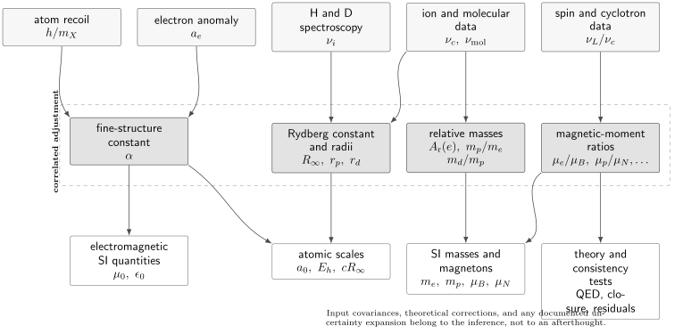
AMO constant determinations form an observational network. Arrows represent both exact identities and theory-dependent observational equations; a global adjustment must retain their covariance and theoretical corrections.

Correlated Least-Squares Adjustment

Linearization and the normal equations

Suppose the measured input vector has covariance matrix $V_y$. Near a reference point $\mathbf x_0$, linearize the observational equations:

$$\mathbf f(\mathbf x) \simeq \mathbf f(\mathbf x_0) + A\,\delta\mathbf x, \qquad A_{ij} = \left. \frac{\partial f_i}{\partial x_j} \right|_{\mathbf x_0}.$$

With

$$\mathbf d = \mathbf y-\mathbf f(\mathbf x_0),$$

the generalized least-squares estimate minimizes

$$\chi^2 = \left( \mathbf d-A\delta\mathbf x \right)^{\mathsf T} V_y^{-1} \left( \mathbf d-A\delta\mathbf x \right).$$

When the normal matrix is nonsingular,

$$\widehat{\delta\mathbf x} = \left( A^{\mathsf T}V_y^{-1}A \right)^{-1} A^{\mathsf T}V_y^{-1}\mathbf d,$$

and, in the linear-Gaussian approximation,

$$V_x = \left( A^{\mathsf T}V_y^{-1}A \right)^{-1}.$$

The off-diagonal elements of $V_x$ are part of the result. A later calculation involving two adjusted constants must use

$$u^2(g) = \boldsymbol\nabla g^{\mathsf T} V_x \boldsymbol\nabla g,$$

not add the two quoted marginal uncertainties in quadrature while silently setting their correlation to zero.

Why correlations arise

Correlations enter at several levels:

1. Two frequencies may share the same clock, comb, magnetic-field calibration, or line-shape model.
2. Several theoretical predictions may share an uncalculated QED coefficient or a nuclear radius.
3. One input value may already be a least-squares result with internal covariance.
4. The adjustment itself couples constants because one observable depends on several of them.

For example, hydrogen spectroscopy determines a narrow combination of $R_\infty$ and $r_p$, so the adjusted values can be strongly correlated even if the raw transition measurements were independent. Ignoring that correlation can make a derived transition prediction look either artificially precise or artificially uncertain.

Residuals, inconsistency, and uncertainty expansion

For input $i$, a normalized residual is schematically

$$r_i = \frac{ y_i-f_i(\widehat{\mathbf x}) }{ u_i^{\mathrm{eff}} },$$

where $u_i^{\mathrm{eff}}$ must include the relevant covariance with the adjusted prediction. Large residuals signal that the adopted uncertainty model does not describe the input set well.

CODATA may apply a common expansion factor to selected uncertainties before the final adjustment. This is an explicit, documented response to inconsistent data. It does not identify which experiment is biased, erase the disagreement, or convert incompatible results into independent confirmation.

In the 2022 adjustment:

• uncertainties of six leading fine-structure-constant inputs were multiplied by $2.5$;
• the unexpanded normalized residual of the 2018 caesium recoil result was about $4.7$; and
• uncertainties of selected hydrogen and deuterium transition data were multiplied by $1.7$ because their scatter exceeded the adopted model.

These facts belong beside the recommended numbers whenever the result is used as evidence for consistency.

Which adjustment is current?

As of 25 July 2026, the NIST Fundamental Constants Data Center lists CODATA 2022 as the current internationally recommended set. Its input cutoff was 31 December 2022. The next regular adjustment is CODATA 2026, whose data cutoff is 31 December 2026; it is therefore not yet available.

Newer measurements can be more precise than the current recommendation and can foreshadow a future adjustment. They should be labelled post-CODATA 2022, not silently substituted into a table headed “recommended constants.”

Selected CODATA 2022 values

The following rounded values are useful for discussing the inference network. Use the Constants table or the official NIST database for machine-facing work.

Quantity	CODATA 2022 value	Relative standard uncertainty
$\alpha^{-1}$	$137.035\,999\,177(21)$	$1.5\times10^{-10}$
$R_\infty$	$10\,973\,731.568\,157(12)\ {\rm m^{-1}}$	$1.1\times10^{-12}$
$m_p/m_e$	$1836.152\,673\,426(32)$	$1.7\times10^{-11}$
$\mu_e/\mu_B$	$-1.001\,159\,652\,180\,46(18)$	$1.8\times10^{-13}$
$\mu_p/\mu_N$	$2.792\,847\,344\,63(82)$	$2.9\times10^{-10}$
$\mu_n/\mu_N$	$-1.913\,042\,76(45)$	$2.4\times10^{-7}$

The digits in parentheses are one-standard-deviation uncertainties in the last quoted digits. They are marginal uncertainties; they do not display the correlations among entries.

Fine-Structure Constant

Physical role and present SI role

The fine-structure constant sets the dimensionless strength of the electromagnetic interaction:

$$\alpha = \frac{e^2}{4\pi\epsilon_0\hbar c} \simeq \frac{1}{137}.$$

In nonrelativistic atomic physics, it relates characteristic scales:

$$\frac{v_{\mathrm{Bohr}}}{c} \sim \alpha, \qquad \frac{E_{\mathrm{fine}}}{E_{\mathrm{gross}}} \sim \alpha^2.$$

In QED it is the perturbative expansion parameter, although coefficients, logarithms, bound-state factors such as $Z\alpha$, and nonperturbative effects determine the accuracy of any particular truncation.

Because $e$, $h$, and $c$ are exact in the current SI,

$$\mu_0 = \frac{2\alpha h}{e^2c}$$

is now an experimentally inferred quantity. Statements that $\mu_0$ is exact refer to the pre-2019 SI.

Atom-recoil route

Combining

$$R_\infty = \frac{\alpha^2m_ec}{2h}$$

with the relative atomic masses

$$A_{\mathrm r}(X) = \frac{m_X}{m_u}, \qquad A_{\mathrm r}(e) = \frac{m_e}{m_u},$$

gives the recoil observational equation

$$\alpha^2 = \frac{2R_\infty}{c} \frac{A_{\mathrm r}(X)}{A_{\mathrm r}(e)} \frac{h}{m_X}.$$

An atom interferometer measures the response to known photon momentum. For a two-level momentum separation $\hbar k$, the single-photon recoil angular frequency is

$$\omega_r = \frac{\hbar k^2}{2m_X}.$$

Large-momentum-transfer pulses or Bloch oscillations amplify the phase associated with $h/m_X$. The final value of $\alpha$ also requires $A_{\mathrm r}(X)/A_{\mathrm r}(e)$ and $R_\infty$. The method is largely independent of the electron-anomaly route, which makes the comparison especially valuable.

The leading experimental issues include:

• wavefront curvature and Gouy phase, which change the effective photon momentum;
• spatial sampling of the optical field by a finite-temperature cloud;
• gravity gradients, Coriolis acceleration, and trajectory mismatch;
• light shifts, diffraction phases, and pulse imperfections;
• refractive-index corrections from background atoms; and
• atomic-mass and binding-energy inputs.

The sensor-level treatment is developed in Atom-Interferometric Sensors.

Electron magnetic anomaly route

For a free electron,

$$\boldsymbol\mu_e = g_e \frac{q_e}{2m_e} \mathbf S, \qquad a_e = \frac{|g_e|-2}{2}.$$

The Standard Model prediction can be organized as

$$a_e^{\mathrm{SM}} = \sum_{n\geq1} C_n \left( \frac{\alpha}{\pi} \right)^n + a_e^{\mathrm{had}} + a_e^{\mathrm{weak}} + \delta a_e^{\mathrm{mass}},$$

where the coefficients include mass-dependent QED contributions and the last terms collect hadronic, weak, and residual mass-ratio effects. A Penning-trap experiment measures the anomaly from the difference or ratio of spin-precession and cyclotron frequencies. Inverting the theoretical series gives $\alpha$.

This route is extraordinarily sensitive, but it is not theory-free. The inference uses high-order QED coefficients, hadronic and electroweak contributions, and auxiliary mass ratios. Conversely, inserting an independent recoil value of $\alpha$ turns the electron anomaly into a stringent Standard Model test.

The present high-precision comparison

Route	Reported inverse fine-structure constant	Relative uncertainty	Status
Cs recoil, Parker et al. (2018)	$137.035\,999\,046(27)$	$2.0\times10^{-10}$	CODATA input
Rb recoil, Morel et al. (2020)	$137.035\,999\,206(11)$	$8.1\times10^{-11}$	CODATA input
Electron anomaly, Fan et al. (2023) plus SM theory	$137.035\,999\,166(15)$	$1.1\times10^{-10}$	CODATA input
CODATA 2022 adjusted value	$137.035\,999\,177(21)$	$1.5\times10^{-10}$	Current recommendation

The caesium and rubidium recoil values differ by

$$\Delta\alpha^{-1} = 160\times10^{-9},$$

while their original combined standard uncertainty is approximately

$$u_c = \sqrt{27^2+11^2}\times10^{-9} \simeq 29.2\times10^{-9}.$$

Their pairwise separation is therefore about $5.5$ standard deviations if the published uncertainties are treated as independent. Shared adjusted inputs make the full CODATA comparison slightly more subtle, but do not remove the experimental tension. The $2.5$ uncertainty expansion in the 2022 adjustment is why the recommended uncertainty is larger than a naive weighted average would suggest.

The correct conclusion is not that one route has already failed. It is that the highest-precision determinations do not yet constitute a mutually consistent ensemble at their original stated uncertainties. Independent recoil geometries, atomic species, electron-anomaly measurements, and theory cross-checks remain scientifically important.

What an alpha result must report

A reusable determination should separate:

1. the primary measured quantity, such as $h/m_X$ or $a_e$;
2. the observational equation and convention;
3. auxiliary constants and the CODATA edition used;
4. theory contributions and their covariance;
5. statistical and systematic uncertainty components;
6. correlations with earlier measurements;
7. blind-analysis or reversal procedures; and
8. both the direct observable and the converted $\alpha$ value.

Reporting only $\alpha^{-1}$ makes later re-evaluation unnecessarily difficult when a mass, theory coefficient, or recommended constant changes.

Rydberg Constant

Energy scale and adjusted role

The Rydberg constant is related to the electron mass and fine-structure constant by

$$R_\infty = \frac{\alpha^2m_ec}{2h},$$

or, equivalently,

$$hcR_\infty = \frac{E_h}{2}.$$

It sets the leading electronic binding-energy scale for an infinitely heavy, pointlike nucleus. The subscript $\infty$ refers to the infinite-nuclear-mass limit; actual atomic levels include reduced-mass, relativistic, radiative, recoil, and finite-size corrections.

The exact identity does not make $R_\infty$ exact. In the present SI, $h$ and $c$ are exact, whereas $\alpha$ and $m_e$ are adjusted. In the CODATA inference network it is convenient to adjust $R_\infty$ using spectroscopy and connect it to other constants through observational equations.

Hydrogen is a coupled inference

A schematic hydrogen level can be written

$$\begin{aligned} E_{n\ell j} = hcR_\infty \bigg[ & f_{nj}^{\mathrm{Dirac}} \left( \alpha,\frac{m_p}{m_e} \right) \\ & + f_{n\ell j}^{\mathrm{QED}} \left( \alpha,\frac{m_p}{m_e},\ldots \right) \\ & + \delta_{\ell0} \frac{C_{\mathrm{NS}}}{n^3}r_p^2 + \cdots \bigg]. \end{aligned}$$

Here $f^{\mathrm{Dirac}}$ includes the reduced-mass relativistic spectrum, $f^{\mathrm{QED}}$ includes radiative, recoil, hadronic, and weak contributions at the adopted order, and the displayed nuclear-size term is the leading $S$-state contribution. A transition obeys

$$h\nu_{a\to b} = E_b-E_a.$$

At leading nonrelativistic order,

$$\nu_{n_a\to n_b} \simeq cR_\infty \left( \frac{1}{n_a^2} - \frac{1}{n_b^2} \right),$$

but this formula is not adequate for a precision determination. The proton-radius contribution and leading Lamb-shift terms both have approximately $n^{-3}$ scaling for $S$ states. Consequently, one transition generally constrains a combination of $R_\infty$, $r_p$, and QED terms rather than isolating one constant.

Two transitions with sufficiently different sensitivity vectors can determine $R_\infty$ and $r_p$ under an adopted theory model. A third independent transition can then test that model. Alternatively, a precise proton radius from muonic hydrogen can be supplied as external input, allowing an electronic-hydrogen transition to determine $R_\infty$ more directly.

Sensitivity and correlation

For transition $i$, linearize around reference values:

$$\delta\nu_i = K_{iR}\,\delta R_\infty + K_{ir}\,\delta r_p^2 + \sum_k K_{ik}\,\delta q_k.$$

The $q_k$ represent additional constants or theoretical remainder parameters. If two transitions have nearly proportional rows

$$\left( K_{iR},K_{ir} \right),$$

their combination is poorly conditioned: one direction in $(R_\infty,r_p^2)$ space is tightly determined and the orthogonal direction is not. The fitted constants then have a large correlation coefficient,

$$\rho_{Rr} = \frac{ \operatorname{cov}(R_\infty,r_p^2) }{ u(R_\infty)u(r_p^2) }.$$

Publishing only the two marginal uncertainties hides this geometry.

Current recommendation and newer hydrogen data

CODATA 2022 recommends

$$R_\infty = 10\,973\,731.568\,157(12)\ {\rm m^{-1}}.$$

The adjustment expanded selected hydrogen and deuterium transition uncertainties by $1.7$ to address their scatter.

A post-CODATA 2022 result by Maisenbacher and collaborators measured the hydrogen $2S$–$6P$ transition as

$$\nu_{2S\text{--}6P} = 730\,690\,248\,610.79(48)\ {\rm kHz}.$$

Combining it with the hydrogen $1S$–$2S$ frequency gave

$$\begin{aligned} r_p &= 0.8406(15)\ {\rm fm}, \\ R_\infty &= 10\,973\,731.568\,152(14)\ {\rm m^{-1}}, \end{aligned}$$

with a reported correlation of approximately $0.94$ between the inferred $r_p$ and $R_\infty$. Using the muonic-hydrogen radius as an input instead gave

$$R_\infty = 10\,973\,731.568\,1524(79)\ {\rm m^{-1}}.$$

This latter uncertainty is smaller than the CODATA 2022 uncertainty, and the central values are compatible. The result also tests the Standard Model prediction for the measured transition at $0.7$ parts per trillion and the relevant bound-state QED contribution at about $0.5$ parts per million.

These are important 2026 experimental inferences, not a CODATA 2026 recommendation. The distinction matters because a global adjustment must evaluate all eligible post-cutoff data, their correlations, and any updated theory.

Systematics and theory limitations

Hydrogen spectroscopy at this level depends on:

• first- and second-order Doppler effects and the velocity distribution;
• quantum-interference and line-pulling effects among nearby resonances;
• ac and dc Stark shifts, Zeeman shifts, and blackbody radiation;
• frequency-reference and comb traceability;
• recoil and reduced-mass corrections;
• proton charge and magnetic structure;
• correlated bound-state QED remainders; and
• the line-shape model used to map detected counts to an unperturbed frequency.

The Rydberg Formula provides the historical and leading-order spectral structure. It should not be substituted for the full observational equation in a modern constant determination.

Electron-to-Proton Mass Ratio

A convention worth stating

Both

$$\mu_{pe} = \frac{m_p}{m_e}$$

and its inverse

$$\beta_{ep} = \frac{m_e}{m_p}$$

occur in the literature. The symbol $\mu$ is also used for reduced mass and magnetic moment, so a precision report should define its notation explicitly. CODATA 2022 gives

$$\begin{aligned} \frac{m_p}{m_e} &= 1836.152\,673\,426(32), \\ \frac{m_e}{m_p} &= 5.446\,170\,214\,889(94)\times10^{-4}. \end{aligned}$$

These are dimensionless ratios. The proton and electron masses in kilograms additionally depend on the SI realization and the atomic mass constant.

Cyclotron-frequency mass spectrometry

An ideal ion of mass $m$ and charge $q$ in a uniform magnetic field has free cyclotron frequency

$$\nu_c = \frac{|q|B}{2\pi m}.$$

For two ions measured in the same field,

$$\frac{m_1}{m_2} = \frac{|q_1|}{|q_2|} \frac{\nu_{c,2}}{\nu_{c,1}}.$$

The magnetic field cancels only to the extent that the two frequencies sample the same field in time and space. Precision experiments alternate or simultaneously store ions, interpolate magnetic-field drift, control trap anharmonicities, and compare motional energies.

In a real Penning trap, the electrostatic potential splits the motion into modified cyclotron, axial, and magnetron modes. The Brown–Gabrielse invariance theorem gives, to first order in important trap imperfections,

$$\nu_c^2 = \nu_+^2+\nu_z^2+\nu_-^2.$$

The measured ion mass is not automatically the neutral-atom, nuclear, or bare-particle mass needed by an adjustment. For an ion with $N_e$ remaining electrons,

$$m_{\mathrm{ion}}c^2 = m_{\mathrm{nucleus}}c^2 + N_em_ec^2 - E_{\mathrm{bind}},$$

with the sign convention that $E_{\mathrm{bind}}>0$. Electron binding energies, ionization energies, molecular dissociation energies, and their uncertainties must be applied at the precision of the mass ratio.

Bound-electron g-factor route

The electron mass is too small for the most precise direct comparison with ordinary heavy reference ions. A powerful alternative stores a hydrogenlike ion and measures both its cyclotron frequency and the Larmor frequency of its bound electron.

For ion charge $q_{\mathrm{ion}}$ and mass $m_{\mathrm{ion}}$,

$$\nu_c = \frac{|q_{\mathrm{ion}}|B}{2\pi m_{\mathrm{ion}}},$$

while the bound-electron spin frequency is

$$\nu_L = \frac{|g_{\mathrm{bound}}|eB}{4\pi m_e}.$$

Their ratio gives

$$\frac{m_e}{m_{\mathrm{ion}}} = \frac{|g_{\mathrm{bound}}|}{2} \frac{e}{|q_{\mathrm{ion}}|} \frac{\nu_c}{\nu_L}.$$

The cancellation of $B$ is experimental; the extraction of $m_e$ is theory-dependent through $g_{\mathrm{bound}}$. That calculation includes Dirac binding, radiative, recoil, nuclear-size, and nuclear-polarization terms. Sturm and collaborators used this route with hydrogenlike $^{12}\mathrm C^{5+}$ to determine the electron’s relative atomic mass.

Molecular-ion spectroscopy

The rovibrational energies of a light molecular ion depend strongly on nuclear-to-electron mass ratios. In a Born–Oppenheimer scaling estimate,

$$E_{\mathrm{vib}} \propto \mu_{\mathrm{nuc}}^{-1/2}, \qquad E_{\mathrm{rot}} \propto \mu_{\mathrm{nuc}}^{-1},$$

where $\mu_{\mathrm{nuc}}$ is an appropriate nuclear reduced mass in electron-mass units. Thus

$$\frac{\partial\ln\nu_{\mathrm{vib}}} {\partial\ln(m_p/m_e)} \sim -\frac12, \qquad \frac{\partial\ln\nu_{\mathrm{rot}}} {\partial\ln(m_p/m_e)} \sim -1$$

in simple limiting models. Actual three-body calculations include nonadiabatic, relativistic, radiative, finite-size, spin, and external-field effects.

For transition $i$ in a molecular hydrogen ion, write

$$\nu_i^{\mathrm{th}} = cR_\infty F_i \left( \frac{m_p}{m_e}, \frac{m_d}{m_e}, r_p,r_d,\alpha,\ldots \right).$$

The measurement constrains the parameter combination to which $F_i$ is sensitive. A statement that spectroscopy “measured the proton mass” is therefore incomplete unless it specifies the other fixed or adjusted inputs and the ab initio theory covariance.

High-accuracy $HD^+$ work has provided an independent spectroscopic route. Patra and collaborators measured a $v=0\to9$ overtone with a fractional frequency uncertainty of $2.9$ parts per trillion and inferred $m_p/m_e$ at a fractional uncertainty of about $21$ parts per trillion. CODATA 2022 included molecular-hydrogen-ion spectroscopy in its mass adjustment.

In 2025, Alighanbari and collaborators measured an $\mathrm H_2^+$ rovibrational transition with an $8\times10^{-12}$ fractional uncertainty. Their restricted least-squares analysis obtained

$$\left[ \frac{m_p}{m_e} \right]_{\mathrm{H_2^+}} = 1836.152\,673\,414(47),$$

consistent with both CODATA 2022 and the independent $HD^+$ route. This post-CODATA result had a smaller uncertainty than the earlier bound-electron-$g$-factor determination, although not smaller than the CODATA 2022 global-adjustment uncertainty.

The value is a spectroscopic inference under the adopted molecular, hydrogen, and muonic-hydrogen theory inputs. That dependence is a feature: agreement between mass spectrometry, bound-electron spin resonance, and molecular spectroscopy tests a much wider network than repeated use of one apparatus class.

A mass-ratio result is a closure test

Suppose three independent routes determine

$$\frac{m_p}{m_e}, \qquad \frac{m_d}{m_p}, \qquad \frac{m_d}{m_e}.$$

They must satisfy

$$\frac{m_d}{m_e} = \frac{m_d}{m_p} \frac{m_p}{m_e}.$$

Define the logarithmic closure residual

$$\Delta_{\mathrm{cl}} = \ln\!\left(\frac{m_d}{m_e}\right) - \ln\!\left(\frac{m_d}{m_p}\right) - \ln\!\left(\frac{m_p}{m_e}\right).$$

Its uncertainty must include cross-covariances. A statistically significant nonzero value could indicate an experimental bias, a binding energy error, an incomplete theory model, or genuinely new physics. Closure alone does not identify the cause.

Magnetic Moments

Magnetons and g factors

The Bohr and nuclear magnetons are

$$\mu_B = \frac{e\hbar}{2m_e}, \qquad \mu_N = \frac{e\hbar}{2m_p}.$$

They are convenient scale units, not independently adjusted particle moments. Since they contain $m_e$ and $m_p$, their SI values inherit mass uncertainties even though $e$ and $h$ are exact.

For angular momentum $\mathbf J$, define

$$\boldsymbol\mu = g_J\mu_{\mathrm{ref}} \frac{\mathbf J}{\hbar}, \qquad H_Z = -\boldsymbol\mu\mathbin{\cdot}\mathbf B.$$

The reference magneton and charge-sign convention must be stated. For an electron, $q_e=-e$, so its magnetic moment is antiparallel to its spin for positive $|g_e|$. CODATA tabulates the signed ratio

$$\frac{\mu_e}{\mu_B} = -1.001\,159\,652\,180\,46(18).$$

For a nucleus of spin $I$,

$$\boldsymbol\mu_I = g_I\mu_N \frac{\mathbf I}{\hbar}.$$

The proton has

$$\frac{\mu_p}{\mu_N} = 2.792\,847\,344\,63(82),$$

whereas the neutron has a negative moment. Composite-particle $g$ factors encode internal strong-interaction structure; they are not fixed by spin alone.

Magnetic Moments and g Factors owns the general angular-momentum conventions and Zeeman Hamiltonians. Here the emphasis is their determination as constants.

Larmor-to-cyclotron ratio

For a free spin-$1/2$ particle with charge $q$ and mass $m$,

$$\omega_L = |g| \frac{|q|B}{2m}, \qquad \omega_c = \frac{|q|B}{m}.$$

Therefore,

$$\frac{|g|}{2} = \frac{\omega_L}{\omega_c}.$$

The ratio cancels the magnetic field to first order. In a high-precision trap, however, the spin transition and motional frequencies may be measured in different trap regions or at different times. Magnetic-field drift, image-charge shifts, relativistic motional shifts, electric-field imperfections, and spin-state detection all enter the uncertainty budget.

The 2023 free-electron measurement reported

$$\frac{-\mu_e}{\mu_B} = \frac{|g_e|}{2} = 1.001\,159\,652\,180\,59(13).$$

CODATA combines it with theory and other input data rather than simply copying this number into every related entry.

For the proton, a double-trap method separates precision frequency measurement in a homogeneous field from spin-state analysis in a strong magnetic bottle. Schneider and collaborators obtained

$$\frac{\mu_p}{\mu_N} = 2.792\,847\,344\,62(82)$$

at $0.3$ parts per billion. The last displayed digit of the CODATA 2022 adjusted value differs because the recommendation comes from a correlated network and uses its own rounding.

Free, bound, and shielded moments

A magnetic moment measured in an atom, molecule, liquid, or solid is not automatically the free-particle moment. Electronic currents shield the local field at a nucleus:

$$\mathbf B_{\mathrm{loc}} = \left( \mathbf 1-\boldsymbol\sigma \right) \mathbf B_{\mathrm{ext}},$$

where $\boldsymbol\sigma$ is generally a tensor. In an isotropic sample,

$$\mu' = \left( 1-\sigma \right)\mu$$

defines a shielded moment $\mu'$. Extracting $\mu$ requires a calculated or independently measured shielding correction.

A high-precision NMR ratio must therefore state:

• the molecule or material and isotopic composition;
• chemical state, solvent, concentration, and temperature;
• sample shape and demagnetization convention;
• whether the quoted quantity is free, bound, or shielded;
• the shielding calculation and its uncertainty; and
• correlations introduced by a common reference sample.

Labels such as “proton moment in water at $25\,^\circ\mathrm C$” are not decorative metadata. They define the measurand.

Hyperfine spectroscopy

For an $S$ electron, the leading Fermi-contact interaction has the form

$$H_{\mathrm F} \propto \boldsymbol\mu_e \mathbin{\cdot} \boldsymbol\mu_I |\psi(0)|^2.$$

The corresponding hyperfine interval is sensitive to a product of magnetic moments and the wavefunction at the nucleus. A precision prediction also includes relativistic, radiative, recoil, nuclear magnetization-distribution, nuclear polarizability, and finite-charge-size corrections.

Consequently, hyperfine spectroscopy can determine a moment ratio only after atomic or molecular structure theory separates these contributions. For hydrogen, the Zemach radius and proton polarizability become limiting nuclear-structure terms. For many-electron atoms, electronic correlation and shielding can dominate. A precise interval is not by itself a theory-independent free nuclear moment.

Moment ratios and conversion chains

Experiments often compare two moments more directly than either absolute moment:

$$\frac{\mu_A}{\mu_B} = \frac{\nu_A}{\nu_B} \frac{I_A}{I_B} \frac{1-\sigma_B}{1-\sigma_A},$$

schematically for two spin species in a common field. The exact equation depends on whether frequencies, angular frequencies, signs, and spin quantum numbers have been absorbed into the reported ratio.

To convert a measured shielded ratio into $\mu_A/\mu_N$, an adjustment may need:

1. another magnetic-moment ratio;
2. one or more shielding differences;
3. the electron-to-proton mass ratio;
4. the electron anomaly or a bound-electron $g$ factor; and
5. covariance among all these inputs.

This long conversion chain explains why CODATA magnetic-moment tables contain many correlated entries and why a local update can propagate beyond the originally measured species.

Spectroscopy as a Constants Experiment

The forward model

A precision spectrum becomes a constants experiment only through a forward model. For line $i$,

$$\nu_i^{\mathrm{pred}} = \nu_i \left( \mathbf x,\boldsymbol\theta \right),$$

where $\mathbf x$ contains constants of interest and $\boldsymbol\theta$ contains nuisance parameters, field shifts, line-shape parameters, and theoretical remainders. The measured line centre is

$$\nu_i^{\mathrm{obs}} = \nu_i^{\mathrm{pred}} + \Delta_i^{\mathrm{exp}} + \epsilon_i.$$

Here $\Delta_i^{\mathrm{exp}}$ represents applied or fitted experimental corrections and $\epsilon_i$ the residual stochastic error under the adopted model.

The laboratory problem and the constants problem should be separated:

$$\begin{aligned} \text{detector records} &\longrightarrow \widehat{\nu}_i,\ V_\nu, \\ \widehat{\nu}_i,\ V_\nu,\ \text{theory} &\longrightarrow \widehat{\mathbf x},\ V_x. \end{aligned}$$

The first line belongs to frequency metrology and line-shape inference. The second belongs to the constants adjustment. Combining them in one opaque fit can make systematic corrections and shared theory errors difficult to audit.

Logarithmic sensitivity coefficients

For a dimensionless constant $X_a$, define

$$K_{ia} = \frac{\partial\ln\nu_i} {\partial\ln X_a}.$$

Small changes then obey

$$\frac{\delta\nu_i}{\nu_i} = \sum_a K_{ia} \frac{\delta X_a}{X_a} + \frac{\delta\nu_i^{\mathrm{th}}}{\nu_i}.$$

Sensitivity coefficients expose three distinct questions:

• leverage: how much does the line move when a constant changes?
• identifiability: are the sensitivity vectors of available lines linearly independent?
• robustness: does a useful combination suppress a common nuisance or theory term?

A line with a large $|K_{ia}|$ is not automatically the best measurement. It may be broad, field-sensitive, theoretically uncertain, or nearly degenerate with another parameter.

Frequency ratios

For a ratio $R_{ij}=\nu_i/\nu_j$,

$$\delta\ln R_{ij} = \sum_a \left( K_{ia}-K_{ja} \right) \delta\ln X_a.$$

A common dimensional energy scale cancels when $K_{iR}=K_{jR}$. This is why clock and molecular frequency ratios are powerful probes of dimensionless combinations. The cancellation can also reduce sensitivity to a constant one intended to determine, so the ratio must be designed for the scientific target rather than assumed to be universally superior.

Theory uncertainty as data

An uncalculated contribution should not be hidden inside prose. One useful model introduces a theory nuisance parameter $t_k$ with prior covariance $V_t$:

$$\nu_i^{\mathrm{th}} = \nu_{i,0}^{\mathrm{th}} + \sum_k B_{ik}t_k.$$

Marginalizing over $\mathbf t$ contributes

$$V_{\mathrm{th}} = B V_t B^{\mathsf T}$$

to the transition covariance. This automatically preserves shared theory errors across several lines. Treating the same omitted QED coefficient as independent noise in every transition would overstate the information content of the dataset.

Theory errors should be classified:

• numerical convergence or basis-set uncertainty;
• uncertainty propagated from input constants;
• uncertainty in nuclear radii, polarizabilities, or structure;
• truncation of a controlled perturbation series;
• estimated uncalculated terms with shared coefficients; and
• model discrepancy that is not justified by a probabilistic expansion.

The last category should not be assigned a tiny Gaussian uncertainty merely because the fit software requires one.

Designing an identifiable measurement set

Let $K$ be the matrix of sensitivity coefficients and $V$ the total frequency covariance. The local information matrix is

$$\mathcal I = K^{\mathsf T}V^{-1}K.$$

Small eigenvalues of $\mathcal I$ identify poorly constrained combinations of constants. Good experimental design can improve them by selecting:

• transitions with complementary sensitivities;
• isotopologues that change mass and nuclear-size dependence;
• ratios that cancel dominant common shifts;
• field-reversal or state-reversal channels that isolate nuisance terms;
• direct mass or radius inputs that rotate a spectroscopic degeneracy; and
• measurements from independent apparatus classes.

The determinant or condition number of $\mathcal I$ can guide design, but must be interpreted with physically meaningful parameter scaling.

Evidence and Reporting Standards

Minimum record for a determination

A mature constants result should make the following recoverable:

Item	Required content
Measurand	Primary frequency, ratio, recoil quantity, anomaly, or mass ratio
Convention	Signs, charge states, magneton, isotope, free/bound/shielded status
Forward model	Observational equation and theory version
Corrections	Applied value, sign, uncertainty, and evaluation method
Covariance	Shared experimental and theoretical terms
Auxiliary inputs	Numerical values, editions, and persistent references
Fit	Parameters adjusted, priors, residuals, and goodness of fit
Robustness	Reversals, subsets, alternative models, and blind-analysis status
Output	Primary observable plus converted constant and covariance
Reusability	Data, code, or enough numerical detail for re-adjustment

The direct observable should be retained with more digits than the converted headline value. A future adjustment can then update auxiliary constants without reconstructing the experiment from a rounded plot.

Common mistakes

Calling a derived value direct.
Atom recoil directly determines $h/m_X$ through an apparatus model, not $\alpha$ without other inputs. Molecular spectroscopy directly determines a transition frequency, not $m_p/m_e$ without molecular theory.

Using a post-cutoff paper as a new CODATA value.
A precise new result can supersede one input experimentally without superseding the internationally recommended adjustment.

Ignoring covariance.
Two constants quoted on adjacent rows of a table are not generally independent. Nor are two theory predictions that share an omitted coefficient.

Treating uncertainty expansion as agreement.
Expansion makes the adjusted uncertainty more conservative. It does not explain the source of discordant measurements.

Confusing exact and measured SI quantities.
In the current SI, $h$, $e$, and $c$ are exact; $\alpha$, $\mu_0$, and $\epsilon_0$ are not.

Omitting charge and binding corrections.
A Penning trap measures an ion. Converting it to a neutral atom, nucleus, or bare particle requires mass-energy bookkeeping.

Confusing a shielded moment with a free moment.
The chemical and material environment is part of the measurand until a shielding model removes it.

Testing theory with a fitted input.
If a constant was inferred using the same theoretical relation later claimed as a test, the comparison is circular unless an independent input breaks the loop.

Worked Reasoning Patterns

From an observable to a constant

For any proposed determination, write the dependency graph before propagating numbers:

$$\text{raw data} \to \text{primary observable} \to \text{corrected observable} \to \text{observational equation} \to \text{constant}.$$

At each arrow ask:

1. Is it exact, calibrated, fitted, or calculated?
2. Which uncertainty enters?
3. Is that uncertainty shared elsewhere?
4. Can a reversal or independent route test it?

This procedure catches many hidden assumptions before they become sub-parts-per-billion claims.

From a constant to a theory test

To use measurement $A$ as a determination and measurement $B$ as a test:

1. Infer the constant from $A$ using theory terms independent of the one tested in $B$.
2. Propagate the full covariance into the prediction for $B$.
3. Compare the primary observable in $B$ with that prediction.
4. Report the residual in physical units and normalized units.
5. Check whether $A$ and $B$ share calibration, auxiliary data, or theory.

For example, recoil $\alpha$ inserted into the electron anomaly prediction tests high-order QED. Electron-anomaly $\alpha$ inserted back into the same anomaly formula does not.

Exercises

Exercise 1: Derive the recoil observational equation

Starting from

$$R_\infty = \frac{\alpha^2m_ec}{2h},$$

derive an expression for $\alpha^2$ in terms of $R_\infty$, $h/m_X$, $A_{\mathrm r}(X)$, and $A_{\mathrm r}(e)$. Identify which factor an atom-recoil apparatus most directly determines.

Solution

Solve the Rydberg identity for $\alpha^2$:

$$\alpha^2 = \frac{2R_\infty}{c} \frac{h}{m_e}.$$

Insert

$$\frac{h}{m_e} = \frac{h}{m_X} \frac{m_X}{m_e} = \frac{h}{m_X} \frac{A_{\mathrm r}(X)}{A_{\mathrm r}(e)}.$$

Therefore,

$$\alpha^2 = \frac{2R_\infty}{c} \frac{A_{\mathrm r}(X)}{A_{\mathrm r}(e)} \frac{h}{m_X}.$$

The interferometric apparatus most directly determines $h/m_X$, after its phase, wavevector, geometry, and systematic corrections are modelled. $R_\infty$ and the relative masses are auxiliary adjusted inputs.

Exercise 2: Recoil frequency and scaling

For $^{87}\mathrm{Rb}$ at wavelength $\lambda=780\ {\rm nm}$, estimate the single-photon recoil frequency

$$f_r = \frac{\omega_r}{2\pi} = \frac{h}{2m\lambda^2}.$$

Use $m\simeq87u$ and $u=1.66054\times10^{-27}\ {\rm kg}$. Then explain why large momentum transfer is useful when $f_r$ is only a few kilohertz.

Solution

The atomic mass is approximately

$$m \simeq 87(1.66054\times10^{-27}) = 1.4447\times10^{-25}\ {\rm kg}.$$

Hence

$$\begin{aligned} f_r &= \frac{6.62607\times10^{-34}} {2(1.4447\times10^{-25})(780\times10^{-9})^2} \\ &\simeq 3.77\times10^3\ {\rm Hz}. \end{aligned}$$

The recoil itself is small compared with optical frequencies. Coherent transfer of many photon momenta accumulates a phase proportional to a large integer multiple of the recoil, improving statistical leverage. This does not automatically reduce wavefront, diffraction-phase, or trajectory systematics; those can also scale with the pulse sequence.

Exercise 3: Quantify the recoil discrepancy

Treat the 2018 caesium and 2020 rubidium values as independent:

$$\begin{aligned} \alpha_{\mathrm{Cs}}^{-1} &= 137.035\,999\,046(27), \\ \alpha_{\mathrm{Rb}}^{-1} &= 137.035\,999\,206(11). \end{aligned}$$

Compute their difference in units of the combined standard uncertainty. What would multiplying both uncertainties by $2.5$ do to this pairwise normalized separation?

Solution

The absolute difference is

$$\Delta = 160\times10^{-9}.$$

The independent combined uncertainty is

$$u_c = \sqrt{27^2+11^2}\times10^{-9} = 29.15\times10^{-9}.$$

Thus

$$\frac{\Delta}{u_c} \simeq 5.49.$$

If both marginal uncertainties are multiplied by $2.5$, the denominator is also multiplied by $2.5$, giving

$$\frac{5.49}{2.5} \simeq 2.20.$$

This demonstrates what uncertainty expansion does numerically. It reduces the normalized tension used by the adjustment, but it does not discover the cause or make the original experiments agree at their published uncertainties.

Exercise 4: Two-transition conditioning

Consider the linearized model

$$\begin{pmatrix} \delta\nu_1\\ \delta\nu_2 \end{pmatrix} = \begin{pmatrix} 1 & 1\\ 1 & 1+\varepsilon \end{pmatrix} \begin{pmatrix} x\\ y \end{pmatrix},$$

with equal independent frequency uncertainties $\sigma$. Interpret $x$ as a scaled $R_\infty$ shift and $y$ as a scaled $r_p^2$ shift. Solve for $x$ and $y$. How does the uncertainty behave as $\varepsilon\to0$?

Solution

Subtract the two equations:

$$\delta\nu_2-\delta\nu_1 = \varepsilon y,$$

so

$$y = \frac{\delta\nu_2-\delta\nu_1}{\varepsilon}, \qquad x = \delta\nu_1-y.$$

Because the two measurements are independent,

$$u^2(y) = \frac{2\sigma^2}{\varepsilon^2}.$$

Thus $u(y)\propto1/|\varepsilon|$, and the uncertainty of $x$ also diverges. At $\varepsilon=0$, the two sensitivity rows are identical and only $x+y$ is identifiable. The example captures why nominally precise hydrogen transitions can leave $R_\infty$ and $r_p$ highly correlated.

Exercise 5: Charge states and binding energy

Two ions have charges $q_1=5e$ and $q_2=e$. Their measured free-cyclotron frequency ratio is

$$\frac{\nu_{c,2}}{\nu_{c,1}} = 0.400\,000\,000.$$

Find $m_1/m_2$ in the ideal model. Then write the correction needed if ion 1 was formed from a neutral atom by removing five electrons with total ionization energy $E_{\mathrm{ion}}>0$.

Solution

The ideal ratio is

$$\frac{m_1}{m_2} = \frac{5e}{e}(0.400\,000\,000) = 2.000\,000\,000.$$

If neutral atom 1 has mass $m_{1,\mathrm{atom}}$, then

$$m_{1,\mathrm{ion}}c^2 = m_{1,\mathrm{atom}}c^2 - 5m_ec^2 + E_{\mathrm{ion}}.$$

The positive $E_{\mathrm{ion}}$ term appears because removing bound electrons requires energy: the neutral atom’s binding lowers its mass relative to the separated constituents. Therefore,

$$m_{1,\mathrm{atom}} = m_{1,\mathrm{ion}} + 5m_e - \frac{E_{\mathrm{ion}}}{c^2}.$$

The trap ratio determines the ion mass. The electron masses and total ionization energy must be included before quoting the neutral-atom mass.

Exercise 6: Molecular sensitivity

In a simple model, a vibrational transition satisfies

$$\nu_{\mathrm{vib}} \propto \left( \frac{m_p}{m_e} \right)^{-1/2}.$$

If the measured frequency is $60\ {\rm THz}$ with a fractional uncertainty of $3\times10^{-12}$ and all other contributions are exact, estimate the best possible fractional uncertainty in $m_p/m_e$. Why is this only a lower bound for a real molecular-ion determination?

Solution

Taking logarithms gives

$$\delta\ln\nu_{\mathrm{vib}} = -\frac12 \delta\ln\!\left(\frac{m_p}{m_e}\right).$$

Therefore,

$$\frac{ u(m_p/m_e) }{ m_p/m_e } = 2 \frac{u(\nu)}{\nu} = 6\times10^{-12}.$$

This is a lower bound because real theory also depends on $R_\infty$, other nuclear mass ratios, charge radii, $\alpha$, relativistic and QED terms, hyperfine deperturbation, and external-field corrections. Their uncertainties and correlations must be included.

Exercise 7: g factor and sign

A trapped electron has measured magnitude ratio

$$\frac{\omega_L}{\omega_c} = 1.001\,159\,652\,18.$$

Find $|g_e|$ and $a_e$. Why is the signed ratio $\mu_e/\mu_B$ negative even though both numbers just calculated are positive?

Solution

Since

$$\frac{|g_e|}{2} = \frac{\omega_L}{\omega_c},$$

we obtain

$$|g_e| = 2.002\,319\,304\,36.$$

The anomaly is

$$a_e = \frac{|g_e|-2}{2} = 0.001\,159\,652\,18.$$

The electron charge is negative. Its magnetic moment vector is therefore antiparallel to its spin vector under the common convention, so $\mu_e/\mu_B<0$. Frequency magnitudes discard this orientation sign; recovering it requires the declared Hamiltonian and charge convention.

Exercise 8: Propagating a correlated pair

Let a derived quantity be

$$z=x-y.$$

Suppose

$$u(x)=2,\qquad u(y)=3,\qquad \rho_{xy}=0.8.$$

Compute $u(z)$. Compare with the value obtained by incorrectly assuming independence.

Solution

The covariance is

$$\operatorname{cov}(x,y) = \rho_{xy}u(x)u(y) = 0.8(2)(3) = 4.8.$$

For $z=x-y$,

$$\begin{aligned} u^2(z) &= u^2(x)+u^2(y) - 2\operatorname{cov}(x,y) \\ &= 4+9-9.6 = 3.4. \end{aligned}$$

Thus

$$u(z) = \sqrt{3.4} \simeq 1.84.$$

Assuming independence would give

$$u_{\mathrm{ind}}(z) = \sqrt{13} \simeq 3.61.$$

Positive correlation reduces uncertainty in a difference. For a sum, the same covariance would increase it. Dropping covariance is not automatically conservative.

Further Connections

• Precision Measurement and Metrology develops measurands, calibration, corrections, covariance, and validation.
• Precision Spectroscopy follows the path from a spectral signal to a corrected frequency and uncertainty budget.
• Variation of Constants Searches turns sensitivity coefficients and comparison records into drift, modulation, transient, and model-coupling limits.
• Atom-Interferometric Sensors develops recoil phase, scale factors, wavefront effects, and inertial-systematic control.
• Single-Electron Devices develops the quantized-current relation $I=nef$, pump error channels, and the evidence needed to use controlled electron transfer in electrical metrology.
• Atomic Units and Scales explains how $\alpha$, $m_e$, and $R_\infty$ organize atomic length and energy scales.
• Constants and Conversions provides the versioned AMO lookup layer for spectroscopic, magnetic, temperature, and dipole-unit translations.
• Rydberg Formula gives the leading spectral series and its historical role.
• Magnetic Moments and g Factors establishes spin, charge, magneton, and Zeeman conventions.
• Constants provides a concise lookup table and links to the official recommended dataset.

References

Adjustments, SI, and data

1. P. J. Mohr, D. B. Newell, B. N. Taylor, and E. Tiesinga, CODATA recommended values of the fundamental physical constants: 2022, Rev. Mod. Phys. 97, 025002 (2025).
2. P. J. Mohr, D. B. Newell, B. N. Taylor, and E. Tiesinga, CODATA recommended values of the fundamental physical constants: 2022, J. Phys. Chem. Ref. Data 54, 033105 (2025). This parallel publication includes detailed input tables, observational equations, correlations, and adjustment diagnostics.
3. NIST Fundamental Constants Data Center, Current CODATA values and 2026 adjustment schedule.
4. BIPM, The International System of Units, ninth edition, SI Brochure, updated version.
5. R. D. Deslattes, P. J. Mohr, and B. N. Taylor, Introduction to the constants for nonexperts, NIST Fundamental Constants Data Center.

Fine-structure constant

6. R. H. Parker, C. Yu, W. Zhong, B. Estey, and H. Müller, Measurement of the fine-structure constant as a test of the Standard Model, Science 360, 191–195 (2018).
7. L. Morel, Z. Yao, P. Cladé, and S. Guellati-Khélifa, Determination of the fine-structure constant with an accuracy of 81 parts per trillion, Nature 588, 61–65 (2020).
8. X. Fan, T. G. Myers, B. A. D. Sukra, and G. Gabrielse, Measurement of the electron magnetic moment, Phys. Rev. Lett. 130, 071801 (2023).
9. T. Aoyama, T. Kinoshita, and M. Nio, Theory of the anomalous magnetic moment of the electron, Atoms 7, 28 (2019).
10. D. Hanneke, S. Fogwell, and G. Gabrielse, New measurement of the electron magnetic moment and the fine structure constant, Phys. Rev. Lett. 100, 120801 (2008).

Rydberg constant and hydrogen

11. L. Maisenbacher, V. Wirthl, A. Matveev, et al., Sub-part-per-trillion test of the Standard Model with atomic hydrogen, Nature 650, 845–851 (2026).
12. A. Grinin, A. Matveev, D. C. Yost, et al., Two-photon frequency comb spectroscopy of atomic hydrogen, Science 370, 1061–1066 (2020).
13. C. G. Parthey, A. Matveev, J. Alnis, et al., Improved measurement of the hydrogen $1S$–$2S$ transition frequency, Phys. Rev. Lett. 107, 203001 (2011).
14. A. Beyer, L. Maisenbacher, A. Matveev, et al., The Rydberg constant and proton size from atomic hydrogen, Science 358, 79–85 (2017).
15. R. Pohl, A. Antognini, F. Nez, et al., The size of the proton, Nature 466, 213–216 (2010).
16. A. Antognini, F. Nez, K. Schuhmann, et al., Proton structure from the measurement of $2S$–$2P$ transition frequencies of muonic hydrogen, Science 339, 417–420 (2013).

Mass ratios and molecular spectroscopy

17. S. Sturm, F. Köhler, J. Zatorski, et al., High-precision measurement of the atomic mass of the electron, Nature 506, 467–470 (2014).
18. F. Heiße, F. Köhler-Langes, S. Rau, et al., High-precision measurement of the proton’s atomic mass, Phys. Rev. Lett. 119, 033001 (2017).
19. S. Alighanbari, G. S. Giri, F. L. Constantin, V. I. Korobov, and S. Schiller, Precise test of quantum electrodynamics and determination of fundamental constants with $HD^+$ ions, Nature 581, 152–158 (2020).
20. S. Patra, M. Germann, J.-P. Karr, et al., Proton-electron mass ratio from laser spectroscopy of $HD^+$ at the part-per-trillion level, Science 369, 1238–1241 (2020).
21. I. V. Kortunov, S. Alighanbari, M. G. Hansen, et al., Proton–electron mass ratio by high-resolution optical spectroscopy of ion ensembles in the resolved-carrier regime, Nat. Phys. 17, 569–573 (2021).
22. S. Alighanbari, M. R. Schenkel, V. I. Korobov, and S. Schiller, High-accuracy laser spectroscopy of $\mathrm H_2^+$ and the proton–electron mass ratio, Nature 644, 69–75 (2025).
23. D. J. Fink and E. G. Myers, Deuteron-to-proton mass ratio from simultaneous measurement of the cyclotron frequencies of $\mathrm H_2^+$ and $\mathrm D^+$, Phys. Rev. Lett. 127, 243001 (2021).

Magnetic moments

24. G. Schneider, A. Mooser, M. Bohman, et al., Double-trap measurement of the proton magnetic moment at 0.3 parts per billion precision, Science 358, 1081–1084 (2017).
25. A. Mooser, H. Kracke, K. Blaum, et al., Direct high-precision measurement of the magnetic moment of the proton, Nature 509, 596–599 (2014).
26. W. D. Phillips, W. E. Cooke, and D. Kleppner, Magnetic moment of the proton in $\mathrm H_2\mathrm O$ in Bohr magnetons, Metrologia 14, 179–183 (1978).
27. J. L. Flowers, B. W. Petley, and M. G. Richards, A measurement of the nuclear magnetic moment of the proton in water, Metrologia 30, 75–87 (1993).