Atom-Interferometric Sensors

An atom-interferometric inertial sensor infers acceleration, rotation, or a spatial derivative of acceleration from the phase of a matter-wave interferometer. In a three-pulse light-pulse instrument, the leading acceleration phase is

$$\Phi_a = \mathbf k_{\mathrm{eff}} \mathbin{\cdot} \mathbf a\,T^2,$$

but a sensor result is not obtained by dividing one fitted phase by $k_{\mathrm{eff}}T^2$. The measured phase is periodic, the atoms respond to acceleration over a finite time and spatial region, the optical phase reference moves, and acceleration, rotation, gravity gradients, laser wavefronts, and environmental fields can enter the same readout.

A defensible measurement therefore requires an explicit inverse problem:

$$\text{populations} \longrightarrow \text{phase} \longrightarrow \text{physical quantity} \longrightarrow \text{corrected result with uncertainty}.$$

That chain is the subject of this page. The central lesson is metrological: an atom interferometer can supply an exceptionally stable quantum test mass, but it does not eliminate geometry, calibration, environmental modelling, or comparison. Atom sensors complement mechanical, optical, and electromagnetic sensors; which instrument is best depends on the measurand, bandwidth, dynamic environment, averaging time, and required traceability.

Canonical Scope

Atom Interferometry owns atom-optical beam splitters and mirrors, Raman and Bragg momentum transfer, the three-pulse Mach–Zehnder sequence, the propagation–laser phase ledger, sensitivity functions, wave-packet closure, contrast, and state-selective readout. Those derivations are used here rather than repeated.

Precision Measurement and Metrology owns the general measurand, correction, covariance, traceability, and validation framework. Quantum Sensing owns Fisher information, quantum resources, backaction, and decoherence-limited estimation. Interferometry owns the cross-platform instrument concepts. Gravimetry and Inertial Sensing specializes that quantum-estimation layer to matter-wave inertial sensors, including matched SQLs, squeezing, resource boundaries, and information per wall time.

This page owns:

• the map from interferometer phase to acceleration, rotation, gravity, or gravity gradient;
• scale-factor calibration, phase ambiguity, null operation, and dynamic range;
• sensor transfer functions, cycle sampling, and auxiliary-sensor correction;
• absolute gravimetry, effective measurement height, environmental corrections, and comparison;
• differential gradiometry, baseline calibration, common-mode rejection, and tensor conventions;
• atom-interferometric gyroscopy and acceleration–rotation separation;
• sensor-level noise, systematic effects, covariance, and reversal protocols; and
• field operation, hybrid sensing, and the evidence needed for a comparison-ready result.

Conventions and Measurands

Sensor axis and phase sign

Define

$$k_{\mathrm{eff}} = \left| \mathbf k_{\mathrm{eff}} \right|, \qquad \widehat{\mathbf e} = \frac{\mathbf k_{\mathrm{eff}}}{k_{\mathrm{eff}}},$$

and let

$$a = \widehat{\mathbf e} \mathbin{\cdot} \mathbf a_{\mathrm{rel}}$$

be the acceleration of the atomic trajectory relative to the optical phase reference, projected along the sensor axis. For an ideal three-pulse sequence with a linear Raman frequency-difference chirp $\alpha$ in radians per second squared, use

$$\Phi = \left( k_{\mathrm{eff}}a-\alpha \right)T^2 + \Phi_{\mathrm{sys}}.$$

Here $\Phi_{\mathrm{sys}}$ contains all modelled phase shifts not assigned to the intended inertial quantity. Reversing the optical phase convention changes several signs together. A report must therefore state the definitions of $\mathbf k_{\mathrm{eff}}$, $\alpha$, the output port, and the correction sign.

For a stationary vertical gravimeter, it is convenient to point $\widehat{\mathbf e}$ downward and write $g>0$. A null measurement then gives

$$\widehat g = \frac{\widehat\alpha}{k_{\mathrm{eff}}} - \frac{\widehat\Phi_{\mathrm{sys}}} {k_{\mathrm{eff}}T^2}.$$

This formula is only as accurate as the calibrated finite-pulse scale factor, the reference trajectory, and the systematic-phase model.

Rotation and gradient conventions

For launch velocity $\mathbf v$ and angular velocity $\boldsymbol\Omega$, the leading rotation phase in the convention used here is

$$\Phi_\Omega = 2T^2 \boldsymbol\Omega \mathbin{\cdot} \left( \mathbf k_{\mathrm{eff}} \mathbin{\times} \mathbf v \right).$$

Define the acceleration-gradient tensor by

$$\Gamma_{ij} = \frac{\partial a_i}{\partial x_j}.$$

For Newtonian gravity $\mathbf a=-\boldsymbol\nabla U$, so $\Gamma_{ij}=-\partial_i\partial_j U$ is symmetric when the potential is smooth. Poisson’s equation gives

$$\operatorname{tr}\boldsymbol\Gamma = -4\pi G\rho.$$

The trace is therefore approximately zero in a source-free region, not inside matter. Some geodetic literature defines a tensor from derivatives of $U$ rather than $\mathbf a$, reversing this sign. Tensor components without a declared convention are ambiguous.

What an inertial sensor measures

An accelerometer does not generally report an invariant property of the atoms alone. It measures relative motion between freely evolving atomic wave packets and the phase fronts established by lasers, mirrors, or waveguides. A stationary vertical instrument can infer local free-fall acceleration because its retroreflection mirror is supported by the laboratory while the atoms fall. On a moving platform, the same observable contains platform specific force, rotation, attitude, vibration, and gravity through the navigation equations.

Likewise, an absolute gravimeter does not measure one universal value of $g$. Local gravity depends on position, height, time, Earth tides, atmospheric and hydrological mass redistribution, polar motion, and nearby objects. The measurand must include a location, epoch or averaging interval, reference height, tide convention, and environmental correction policy.

From Phase to a Sensor Result

A multiparameter measurement model

One interrogation can be represented locally as

$$\Phi_j = \mathbf K_{a,j} \mathbin{\cdot} \mathbf a + \mathbf K_{\Omega,j} \mathbin{\cdot} \boldsymbol\Omega + \mathbf K_{\Gamma,j} : \boldsymbol\Gamma + b_j + \epsilon_j,$$

where $j$ labels a configuration, $\mathbf K_{a,j}$ and $\mathbf K_{\Omega,j}$ are calibrated response vectors, $\mathbf K_{\Gamma,j}$ is a tensor response, $b_j$ is a nuisance bias, and $\epsilon_j$ is statistical noise. A set of measurements has the compact form

$$\boldsymbol\Phi = \mathbf H\boldsymbol\theta + \mathbf b + \boldsymbol\epsilon.$$

The parameter vector $\boldsymbol\theta$ may contain three acceleration components, three rotation components, selected gradient components, and calibration parameters. Recovering them requires more than counting channels:

1. the columns of $\mathbf H$ must be physically identifiable;
2. the matrix must have adequate rank and conditioning;
3. nuisance parameters must be constrained by calibration or modulation;
4. phase wraps must be assigned consistently; and
5. the covariance of channels and auxiliary records must be retained.

Two nominally orthogonal axes can be nearly redundant after projection onto the same launch velocity or gravity vector. A small singular value of $\mathbf H$ amplifies both noise and calibration error even when every individual phase is precise.

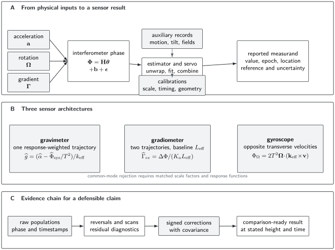
An atom-interferometric sensor is an inverse problem. A: acceleration $\mathbf a$, rotation $\boldsymbol\Omega$, gradients $\boldsymbol\Gamma$, nuisance phases, auxiliary records, and calibrations jointly determine the result. B: gravimeters, gradiometers, and gyroscopes use related interferometers but different combinations of trajectories and response vectors. C: raw populations become a comparison-ready value only after reversals, corrections, covariance propagation, and declaration of the reference time and location.

Calibrated scale factor

For instantaneous pulses and constant acceleration,

$$K_a \equiv \frac{\partial\Phi}{\partial a} = k_{\mathrm{eff}}T^2.$$

Real pulses have finite duration, pulse centers can be asymmetric, the effective wave vector can vary with optical frequency and pointing, and the atoms sample wavefront curvature. A precision result should therefore use

$$K_a^{(\mathrm{cal})} = \frac{\partial\Phi_{\mathrm{model}}}{\partial a}$$

from the actual pulse timing and validated response model. The uncertainty of $K_a^{(\mathrm{cal})}$ is a multiplicative uncertainty in the inferred acceleration:

$$\frac{u(a)}{|a|} \supset \frac{u(K_a)}{|K_a|}.$$

Timing, optical frequency, beam angle, refractive index along the optical path, chirp synthesis, and electronic delay can all enter this calibration. A wavelength traceable to a frequency reference does not by itself calibrate beam alignment or pulse timing.

Periodic readout and dynamic range

A balanced two-port interferometer has an output of the form

$$P = \frac{1}{2} + \frac{C}{2} \cos \left( \Phi+\phi_{\mathrm{off}} \right),$$

so one population measurement determines phase only modulo $2\pi$ and has poor slope near a fringe maximum or minimum. The acceleration interval corresponding to one full fringe is

$$\Delta a_{2\pi} = \frac{2\pi}{K_a}.$$

For counterpropagating Raman beams near $780\ \mathrm{nm}$, $k_{\mathrm{eff}}\simeq1.61\times10^7\ \mathrm{m}^{-1}$. With $T=0.10\ \mathrm{s}$,

$$K_a \simeq 1.61\times10^5\ \frac{\mathrm{rad}}{\mathrm{m\,s^{-2}}},$$

and

$$\Delta a_{2\pi} \simeq 3.90\times10^{-5}\ \mathrm{m\,s^{-2}}.$$

An unmodelled vibration much larger than this can move the result through many fringes. High sensitivity and unambiguous dynamic range are therefore different performance metrics.

Common operating strategies include:

• applying an analysis phase to alternate between both sides of the fringe;
• servoing the chirp or mirror phase so the residual stays near midfringe;
• using an auxiliary accelerometer to predict the integer fringe index;
• fitting a parametric fringe against a deliberately scanned phase;
• using quadrature channels or simultaneous interferometers; and
• using a sequential Bayesian or Kalman estimator that carries the phase posterior between cycles.

Each strategy has a failure mode. A servo can hide cycle slips, an auxiliary sensor can have delay or scale error, and a nonlinear estimator can become biased when its likelihood or wrap prior is wrong. Raw populations, applied phases, residuals, and wrap decisions should be retained.

Midfringe and null operation

Choose $\phi_{\mathrm{off}}$ so the nominal phase lies at quadrature. For a small residual $\delta\Phi$,

$$\delta P \simeq \pm \frac{C}{2} \delta\Phi.$$

Null operation steers a controlled parameter, such as $\alpha$, until $\delta P$ averages to zero. This is attractive because the result is encoded in a calibrated frequency ramp rather than a large open-loop phase. It does not remove additive systematic phases:

$$\alpha_{\mathrm{null}} = k_{\mathrm{eff}}a + \frac{\Phi_{\mathrm{sys}}}{T^2}.$$

Changing $T$, reversing $\mathbf k_{\mathrm{eff}}$, or modulating a source mass helps separate terms, but only when the parity and scaling of every relevant nuisance effect are included.

Time-Dependent Acceleration

Triangular response kernel

For ideal instantaneous pulses at $0$, $T$, and $2T$, the scalar acceleration phase is

$$\Phi_a = k_{\mathrm{eff}} \int_0^{2T} f(t)a(t)\,dt,$$

with

$$f(t) = \begin{cases} t, & 0<t<T,\\ 2T-t, & T<t<2T,\\ 0, & \text{otherwise}. \end{cases}$$

Thus the instrument reports a time-weighted acceleration, not an instantaneous sample at $t=T$. With the Fourier convention $a(t)=\int \widetilde a(\omega)e^{-i\omega t}\,d\omega/(2\pi)$, the transfer function is

$$\begin{aligned} H_a(\omega) &= k_{\mathrm{eff}} \int_0^{2T} f(t)e^{-i\omega t}\,dt \\ &= k_{\mathrm{eff}} e^{-i\omega T} \left[ \frac{2\sin(\omega T/2)}{\omega} \right]^2. \end{aligned}$$

It obeys $H_a(0)=k_{\mathrm{eff}}T^2$ and has zeros at nonzero $\omega=2\pi n/T$. Finite pulses alter the high-frequency response and must be included when vibration correction is pushed near the pulse bandwidth.

For a two-sided acceleration power spectral density satisfying

$$\left\langle \widetilde a(\omega) \widetilde a^*(\omega') \right\rangle = 2\pi \delta(\omega-\omega') S_a(\omega),$$

the phase variance is

$$\sigma_\Phi^2 = \frac{1}{2\pi} \int_{-\infty}^{\infty} \left| H_a(\omega) \right|^2 S_a(\omega)\,d\omega.$$

One-sided spectra require the corresponding factor-of-two convention. Mixing one-sided and two-sided definitions is a common numerical error.

Cycle sampling and aliasing

If an estimate is produced every cycle time $T_c$, continuous motion noise is sampled at the cycle rate. Spectral components separated by $2\pi/T_c$ can alias into the measurement band. Dead time also means that the instrument is blind during part of each cycle, so the sampled transfer function contains preparation and detection windows in addition to the interferometer kernel.

An auxiliary seismometer or mechanical accelerometer should be transformed through the atom sensor’s response:

$$\widehat\Phi_{\mathrm{vib}} = \int h_a(t-t') a_{\mathrm{aux}}(t')\,dt',$$

not merely sampled at the central pulse. Its gain, phase delay, axis projection, mounting point, self-noise, and saturation must be calibrated. A small timing error can become a large residual where vibration spectra are steep.

Interleaved operation can reduce dead time and increase sampling rate by sharing laser pulses among several clouds. It changes the covariance between successive estimates, so the observed averaging law cannot be interpreted as independent white samples without checking that covariance.

Acceleration and Rotation Sensitivity

Statistical phase baseline

For $N$ independent atoms detected in two output ports at midfringe, binomial projection noise gives the approximate phase uncertainty

$$\sigma_\Phi \gtrsim \frac{1}{C\sqrt N}.$$

The corresponding single-cycle acceleration uncertainty is

$$\sigma_a \gtrsim \frac{1} {C\sqrt N\,K_a}.$$

If cycles are independent and the noise is white, averaging for $\tau\gg T_c$ gives

$$\sigma_a(\tau) \simeq \frac{\sigma_\Phi}{K_a} \sqrt{\frac{T_c}{\tau}}.$$

This is a baseline, not a universal performance law. Atom-number fluctuations, imperfect detection, vibration, oscillator phase, and slow systematics often dominate. Entanglement or spin squeezing can improve the quantum statistical term, but not a wavefront bias or an incorrect reference height.

Acceleration response vector

For a nominal one-axis instrument,

$$\mathbf K_a \simeq T^2\mathbf k_{\mathrm{eff}}.$$

The measured projection depends on attitude. A gravimeter tilted by a small angle $\theta$ from the local vertical measures

$$g_{\mathrm{proj}} = g\cos\theta \simeq g \left( 1-\frac{\theta^2}{2} \right)$$

when horizontal acceleration is negligible. On a moving platform, horizontal specific force leaks into the vertical channel to first order in attitude error. The full calibration is therefore a vector or matrix, not one scalar scale factor.

Axis orthogonality should be measured by rotation, surveying, or a calibrated inertial stimulus. Inferring it only from nominal optical mounts understates alignment uncertainty.

Rotation response vector

Write

$$\mathbf K_\Omega = 2T^2 \left( \mathbf k_{\mathrm{eff}} \mathbin{\times} \mathbf v \right),$$

so that

$$\Phi_\Omega = \mathbf K_\Omega \mathbin{\cdot} \boldsymbol\Omega.$$

The sensor is blind to rotation components orthogonal to $\mathbf K_\Omega$. Three-dimensional rotation sensing therefore requires multiple noncoplanar response vectors or a point-source imaging geometry that maps velocity classes to position-resolved fringes.

For $k_{\mathrm{eff}}=1.61\times10^7\ \mathrm{m}^{-1}$, $T=0.10\ \mathrm{s}$, and transverse speed $v=0.50\ \mathrm{m\,s^{-1}}$,

$$K_\Omega = 2k_{\mathrm{eff}}vT^2 \simeq 1.61\times10^5\ \mathrm{s}.$$

The maximum projection of Earth’s rotation, $\Omega_\oplus\simeq7.292\times10^{-5}\ \mathrm{rad\,s^{-1}}$, would then produce about $11.7\ \mathrm{rad}$. Earth rotation is consequently both a useful calibration signal and a substantial nuisance in gravimetry.

Counterpropagating trajectories

Suppose two interferometers use matched $\mathbf k_{\mathrm{eff}}$ and opposite transverse velocities $\pm\mathbf v$. To leading order,

$$\begin{aligned} \Phi_+ &= K_a a + K_\Omega\Omega + b_+, \\ \Phi_- &= K_a a - K_\Omega\Omega + b_-. \end{aligned}$$

Then

$$\Phi_{\mathrm{sum}} = \frac{\Phi_++\Phi_-}{2}$$

is acceleration-like, while

$$\Phi_{\mathrm{diff}} = \frac{\Phi_+-\Phi_-}{2}$$

is rotation-like. The cancellation fails if the two trajectories have different scale factors, wavefront sampling, launch speeds, pulse timing, contrast, or detection offsets. A gyro uncertainty budget must quantify these mismatches rather than assume parity from the design drawing.

Hybrid inertial sensing

Mechanical accelerometers and optical gyroscopes can have high bandwidth and large dynamic range but slowly drifting bias. Atom interferometers can provide a stable low-frequency reference but usually operate cyclically with limited bandwidth. A complementary estimate can be written

$$\widehat q(s) = H_L(s)\widehat q_{\mathrm{AI}}(s) + H_H(s)\widehat q_{\mathrm{class}}(s),$$

where

$$H_L(s)+H_H(s) \simeq 1$$

over the intended band. Kalman filters formulate the same idea with a state model for classical-sensor bias and atom-sensor observations.

Hybridization is not automatic accuracy transfer. The sensors must refer to matched axes, locations, timestamps, sign conventions, and measurands. Lever arms, relative delay, vibration transfer, scale-factor nonlinearity, and classical-sensor saturation can corrupt the fused result. Validation should include injected motion outside the quiet laboratory regime.

Absolute Gravimetry

Absolute, relative, and conventional

An absolute gravimeter determines acceleration from calibrated time and length or wavelength scales rather than by calibration against another gravimeter. A relative gravimeter measures gravity changes or differences after calibration of its scale factor and drift. Neither label guarantees small uncertainty.

For an atom gravimeter, the primary scale enters through $k_{\mathrm{eff}}$ and pulse timing or chirp. Traceability can involve:

• a frequency reference for the Raman optical frequencies and chirp;
• calibrated timing and phase synthesis;
• surveyed optical geometry and vertical alignment;
• characterization of finite-pulse response;
• a measured vertical gravity gradient and reference height; and
• documented environmental and self-attraction corrections.

International gravimeter comparisons remain essential because no artifact-free point on Earth supplies a fixed natural value of $g$. Comparisons test the complete instrument, including effects that are difficult to establish from component calibrations.

Units and resolution

The SI unit is $\mathrm{m\,s^{-2}}$. Gravimetry also uses

$$\begin{aligned} 1\ \mathrm{Gal} &= 10^{-2}\ \mathrm{m\,s^{-2}}, \\ 1\ \mu\mathrm{Gal} &= 10^{-8}\ \mathrm{m\,s^{-2}}, \\ 1\ \mathrm{E} &= 10^{-9}\ \mathrm{s^{-2}}. \end{aligned}$$

Thus $1\ \mu\mathrm{Gal}$ is about $10^{-9}$ of terrestrial gravity, while one Eötvös is a gradient unit. A phase resolution of $1\ \mathrm{mrad}$ in the numerical example above corresponds to

$$\delta g = \frac{10^{-3}}{1.61\times10^5} \simeq 6.2\times10^{-9}\ \mathrm{m\,s^{-2}} = 0.62\ \mu\mathrm{Gal}.$$

This conversion is a resolution statement. It is not an uncertainty claim until scale factor, bias, and environmental corrections are evaluated.

Response-weighted gravity

When gravity varies along the trajectory and in time, the ideal three-pulse result is

$$g_{\mathrm{eff}} = \frac{1}{T^2} \int_0^{2T} f(t) g[s(t),t]\,dt,$$

where $s$ is a coordinate along the sensor axis. For a locally linear field

$$g(s) = g_r + \Gamma_{ee} \left( s-s_r \right),$$

define the effective measurement coordinate

$$s_{\mathrm{eff}} = \frac{1}{T^2} \int_0^{2T} f(t)s(t)\,dt.$$

For the ideal trajectory

$$s(t) = s_0+v_0t+\frac{1}{2}a_0t^2,$$

the triangular kernel gives

$$s_{\mathrm{eff}} = s_0+v_0T+\frac{7}{12}a_0T^2.$$

Finite pulses, recoil-separated arms, launch geometry, and nonlinear gradients modify this expression. A quoted physical height should be tied to the instrument reference point by a survey and an explicit trajectory model, not inferred from the chamber drawing alone.

To transfer a result from effective height $h_{\mathrm{eff}}$ to a declared reference height $h_r$, use the locally measured vertical gradient:

$$g(h_r) = g(h_{\mathrm{eff}}) + \Gamma_h \left( h_r-h_{\mathrm{eff}} \right),$$

where $\Gamma_h=\partial g/\partial h$ in the chosen upward-height convention. Near Earth’s surface $\Gamma_h$ is usually negative, but local mass distributions can change it. The gradient uncertainty and height uncertainty are correlated contributions to the transferred result.

Environmental and geophysical corrections

Local gravity is time dependent. A stationary series commonly contains signals from:

Effect	Why it enters	Evidence needed
Solid Earth tides	lunar and solar deformation and potential	stated tide model, coordinates, timestamps
Ocean tide loading	elastic response to nearby ocean mass redistribution	loading model and coastal sensitivity
Atmospheric attraction and loading	pressure and three-dimensional air-mass changes	local pressure plus declared admittance or model
Polar motion	centrifugal acceleration changes as Earth’s rotation pole moves	Earth-orientation data and convention
Hydrology	soil moisture, groundwater, snow, and surface water move mass	local sensors or hydrological model when relevant
Vertical gradient	instruments and epochs refer to different heights	measured gradient, survey, transfer equation
Self-attraction	apparatus, platform, vehicles, and operators produce gravity	mass model, configuration control, modulation tests
Nearby construction	elevators, tanks, cranes, and moving masses alter local gravity	site log, exclusion windows, auxiliary monitoring

One must distinguish a correction convention from a physical prediction. For example, a zero-tide result retains the permanent direct effect of the Sun and Moon but removes the permanent deformation term according to the adopted geodetic convention. A comparison report should state the tide system rather than merely say “tides corrected.”

Atmospheric correction based on one local pressure coefficient is often a useful operational approximation, but it does not reproduce all three-dimensional atmospheric loading and attraction. Hydrological corrections can be site-specific and model limited. These residuals can remain correlated over long averaging times.

Instrument corrections in a gravimeter

A representative corrected result is

$$\widehat g_r = \frac{\widehat\alpha}{\widehat k_{\mathrm{eff}}} + \frac{\widehat\Phi_{\mathrm{res}}}{\widehat K_a} - \sum_i c_i + c_h,$$

where $\widehat\Phi_{\mathrm{res}}$ obeys the phase convention declared at the start of the page, $c_i$ are signed instrument and environmental shifts expressed as acceleration, and $c_h$ transfers the response-weighted result to the reference height. An instrument whose electronic error signal has the opposite sign must convert it back to $\Phi_{\mathrm{res}}$ before using this equation. An equally valid ledger adds corrections rather than subtracting shifts. The table and equation must use the same sign.

Important instrument terms include:

• Raman or Bragg wave-vector magnitude and optical-frequency chirp;
• timing, finite-pulse, and electronic-delay corrections;
• beam verticality and retroreflection geometry;
• Coriolis phase from transverse atomic velocity and Earth rotation;
• optical wavefront aberration sampled by the transverse atomic distribution;
• gravity-gradient coupling to launch position and velocity;
• two-photon light shifts, magnetic shifts, and residual frequency detuning;
• source-cloud position, temperature, interactions, and detection inhomogeneity;
• mirror vibration and auxiliary-sensor transfer error; and
• self-attraction by the vacuum system, optical table, support, and nearby masses.

Wavefront error illustrates why source properties belong in the measurement model. If an optical phase surface has local curvature $R^{-1}$, atoms with transverse coordinate $\mathbf r_\perp$ sample a phase roughly proportional to

$$\delta\phi_{\mathrm{wf}} \sim \frac{k_{\mathrm{eff}}} {2R} \left| \mathbf r_\perp \right|^2.$$

The ensemble bias then depends on transverse temperature, expansion time, cloud position, clipping, detection weighting, and pulse-to-pulse wavefront differences. Mapping the wavefront or varying temperature and trajectory provides stronger evidence than assigning a generic optical flatness specification.

Comparison-ready gravity result

A gravity result intended for comparison should report at least:

1. the reference point and physical reference height;
2. coordinates, epoch, averaging interval, and valid data fraction;
3. tide system and geophysical models;
4. instrument configuration, $\mathbf k_{\mathrm{eff}}$ direction, pulse timing, and servo convention;
5. raw and corrected values with a signed correction table;
6. type-A, type-B, and combined standard uncertainties with covariance;
7. vertical-gradient measurement and height transfer;
8. reversals, parameter scans, residual diagnostics, and excluded data;
9. traceability of frequency, time, length, and survey quantities; and
10. comparison results or transport checks where available.

A small Allan deviation is not enough. It establishes a stability property under a stated sampling process, not agreement with the local gravity measurand.

Gravity Gradiometry

Differential measurement and baseline

Two simultaneous atom interferometers at response-weighted positions $\mathbf r_1$ and $\mathbf r_2$ can share the same optical phase reference. For matched acceleration scale factor $K_a$,

$$\Delta\Phi = \Phi_2-\Phi_1 \simeq K_a \widehat{\mathbf e} \mathbin{\cdot} \left( \mathbf a_2-\mathbf a_1 \right) + \Delta\Phi_{\mathrm{sys}}.$$

Let

$$\mathbf L_{\mathrm{eff}} = \mathbf r_{2,\mathrm{eff}} - \mathbf r_{1,\mathrm{eff}}.$$

For a slowly varying gradient,

$$\mathbf a_2-\mathbf a_1 \simeq \boldsymbol\Gamma \mathbf L_{\mathrm{eff}}.$$

If the baseline and sensor axis are both along $\widehat{\mathbf e}$,

$$\widehat\Gamma_{ee} = \frac{ \Delta\Phi-\widehat{\Delta\Phi}_{\mathrm{sys}} }{ K_a L_{\mathrm{eff}} }.$$

The effective baseline is a difference of response-weighted trajectories, not necessarily the distance between trap centers or vacuum-chamber windows.

For $\Gamma_{ee}=3000\ \mathrm E=3.0\times10^{-6}\ \mathrm{s^{-2}}$, $L_{\mathrm{eff}}=1.0\ \mathrm m$, and the preceding $K_a$,

$$\Delta\Phi \simeq (1.61\times10^5) (3.0\times10^{-6}) \simeq 0.483\ \mathrm{rad}.$$

Common-mode rejection and scale mismatch

Shared mirror vibration is rejected only to the extent that the two interferometers have identical response functions. Let

$$\begin{aligned} K_1 &= \overline K-\frac{\delta K}{2}, & K_2 &= \overline K+\frac{\delta K}{2}, \\ a_1 &= \overline a-\frac{\Delta a}{2}, & a_2 &= \overline a+\frac{\Delta a}{2}. \end{aligned}$$

Then

$$K_2a_2-K_1a_1 = \overline K\,\Delta a + \delta K\,\overline a.$$

The second term leaks the large common acceleration into the small differential channel. The same algebra applies to mirror vibration, chirp, and other common inputs. Matching pulse areas but not pulse timing or Rabi frequency can still leave frequency-dependent leakage.

Common-mode rejection should therefore be reported as a transfer function, not one number. Useful tests include injecting mirror motion over frequency, deliberately changing one scale factor, exchanging the two atomic sources, and examining differential residuals against the common channel.

Gradient tensors and closure

A single vertical baseline measures one projection of $\boldsymbol\Gamma$. Reconstructing the full tensor requires several independent axis–baseline combinations and careful treatment of rotations between the instrument and local geodetic frame. In a source-free region, Newtonian theory predicts approximately

$$\Gamma_{ij} = \Gamma_{ji}, \qquad \Gamma_{xx}+\Gamma_{yy}+\Gamma_{zz} \simeq 0.$$

Symmetry and trace closure are valuable diagnostics, but they are not substitutes for calibration. Misalignment, baseline curvature, rotation coupling, and nearby mass inside the measurement region can produce apparent closure failure.

Over a long baseline, the linear approximation can fail:

$$\Delta a_i = \Gamma_{ij}L_j + \frac{1}{2} \frac{\partial\Gamma_{ij}}{\partial x_k} L_jL_k + \cdots.$$

The gradiometer then responds to gradient curvature and to the detailed spatial weighting of both interferometers.

Source masses and Newton’s constant

A modulated source mass can produce a differential phase while common Earth gravity and vibration largely cancel. A schematic model is

$$\Delta\Phi_{\mathrm{near}} = \Delta\Phi_{\mathrm{far}} + K_a \Delta a_{\mathrm{source}}(G,\boldsymbol\eta),$$

where $\boldsymbol\eta$ includes source-mass density, shape, position, atomic trajectories, and baseline. Solving for $G$ requires a gravitational field calculation integrated over the real source and atomic distributions.

The quantum phase can be measured more precisely than the source geometry is known. Density inhomogeneity, positioning, thermal expansion, support structures, trajectory uncertainty, and nearby masses then dominate. Moving the source among several configurations, surveying independently, and fitting one global geometry model provide stronger validation than a single near–far difference.

Gyroscopy and Navigation

Sagnac scale factor

Atom gyroscopes measure a rotation-induced phase associated with the space–time area enclosed by the matter-wave paths. For the simple three-pulse geometry, the response vector

$$\mathbf K_\Omega = 2T^2 \left( \mathbf k_{\mathrm{eff}} \mathbin{\times} \mathbf v \right)$$

shows three routes to larger signal: larger momentum separation, larger transverse speed, and longer interrogation time. Each also tightens requirements on wave-packet closure, beam size, trajectory knowledge, and dynamic control.

The reported angular velocity is

$$\widehat\Omega_e = \frac{ \Phi_{\mathrm{rot}} - \widehat\Phi_{\mathrm{rot,sys}} }{ K_\Omega },$$

where $\Omega_e$ denotes the component along $\mathbf K_\Omega/K_\Omega$. Calibration requires launch velocity, $\mathbf k_{\mathrm{eff}}$, pulse timing, axis orientation, and any finite-pulse correction. A launch-speed drift is a gyro scale-factor drift.

Rotation–acceleration separation

Counterpropagating atomic beams, reversed launch velocities, $\mathbf k_{\mathrm{eff}}$ reversal, and multiple spatial outputs provide different parity channels. Their usefulness depends on a complete parity table:

Contribution	Velocity reversal	Effective-wave-vector reversal
uniform acceleration	even	odd
leading Sagnac rotation	odd	odd
many light shifts	often even	depends on implementation
Coriolis from residual transverse velocity	odd in that velocity	odd
wavefront phase	trajectory dependent	often odd, not guaranteed
detection offset	usually even	usually even

The labels “odd” and “even” are model statements, not experimental facts. Pulse asymmetry or trajectory changes under reversal can mix channels. A global fit to all configurations, with measured scale-factor mismatch, is usually safer than subtracting nominally opposite phases and discarding the sum.

Dynamic operation

Laboratory sensors often assume that the Raman resonance, beam overlap, and phase lie in a narrow operating range. A vehicle introduces:

• large and broadband vibration;
• angular motion during the interrogation;
• time-varying Doppler detuning and beam misalignment;
• Coriolis and centrifugal terms;
• lever-arm acceleration between atom and classical sensors;
• changing gravity and attitude;
• interrupted operation and thermal transients; and
• phase excursions through many fringes.

Long interrogation time increases low-frequency scale factor but narrows the tolerable dynamic envelope. High-rate, interleaved, multi-axis, or guided geometries address parts of this tradeoff. Hybrid classical sensors can preserve phase lock and provide high-rate output, while atom data estimate slow bias.

Navigation performance must be evaluated after integrating sensor errors through the navigation equations. A small acceleration bias produces a velocity error growing approximately linearly with time and a position error growing approximately quadratically before aiding and Earth-frame dynamics are included. Bench-top phase sensitivity alone does not establish navigation accuracy.

Noise and Systematic Effects

A sensor-level ledger

The following categories should be evaluated against the intended measurand:

Source	Coupling to result	Diagnostic or control
Atom projection and detection noise	population uncertainty becomes phase noise	atom-number and contrast scaling, two-port normalization
Laser phase and oscillator noise	pulse phase is sampled directly	independent phase record, common-source test
Mirror vibration	indistinguishable from relative acceleration	isolation, auxiliary sensor, injected-motion transfer test
Timing and chirp synthesis	multiplicative scale and additive phase	calibrated clock, phase-continuity and delay tests
Beam alignment and tilt	projects gravity and platform acceleration	tilt scans, optical survey, attitude sensor
Wavefront aberration	trajectory-dependent optical phase	wavefront map, cloud-position and temperature scans
Coriolis effect	transverse velocity couples to rotation	velocity reversal, launch imaging, orientation scan
Gravity gradients	launch position and velocity become phase	gradient measurement, trajectory scan, compensation
Magnetic fields	Zeeman phase and state-dependent forces	shielding, mapping, field reversal, insensitive states
Optical intensity and detuning	ac Stark shifts and pulse-area changes	intensity extrapolation, detuning reversal, pulse diagnostics
Atom interactions	density-dependent phase or trajectory	density extrapolation, source-state comparison
Detection inhomogeneity	spatial phase is reweighted	imaging, aperture scan, detector model
Self-attraction	apparatus masses alter local gravity	mass model, component movement, independent survey
Dead time and aliasing	high-frequency noise folds into estimates	cycle-timing model, interleaving, spectral injection

A physical effect is not intrinsically “statistical” or “systematic.” Rapid zero-mean vibration can contribute statistical variance; an unmeasured mean tilt is a bias; slowly varying hydrology can be either a signal or a correction depending on the measurand.

Wavefront–trajectory coupling

Let the pulse-dependent transverse optical phase be $\phi_j(\mathbf r_\perp)$. The interferometer contribution is

$$\Phi_{\mathrm{wf}} = \phi_1(\mathbf r_1) - 2\phi_2(\mathbf r_2) + \phi_3(\mathbf r_3).$$

The measured ensemble phase is a nonlinear average over atomic positions, velocities, transition probabilities, and detection weights. It is generally not equal to this expression evaluated at the mean trajectory. Temperature extrapolation can reveal a coupling, but extrapolation to zero temperature is model dependent if clipping or aberrations are nonquadratic. Direct wavefront mapping and controlled trajectory scans provide complementary evidence.

Coriolis and launch velocity

For a vertical gravimeter, Earth rotation produces

$$\Phi_C = 2T^2 \mathbf k_{\mathrm{eff}} \mathbin{\cdot} \left( \mathbf v_\perp \mathbin{\times} \boldsymbol\Omega_\oplus \right).$$

The relevant $\mathbf v_\perp$ is the response-weighted transverse velocity of the detected ensemble. Selection pulses and apertures can make it differ from the mean velocity measured immediately after launch. Reversing launch velocity, rotating the instrument azimuth, and imaging the detected atoms help constrain the model.

Gravity-gradient coupling and closure

In a vertical gradient, the phase depends on initial position and velocity as well as nominal $g$. Schematically,

$$\Phi_\Gamma \sim k_{\mathrm{eff}}\Gamma_{ee} \left( s_0T^2 + v_0T^3 + \cdots \right).$$

The same gradient can prevent perfect phase-space closure and reduce contrast. Changing the effective wave vector of the middle pulse can compensate leading gradient effects in suitable geometries, but the frequency step, actual gradient, and residual higher-order terms become new calibration quantities.

Reversal channels

For effective-wave-vector reversal, define

$$\begin{aligned} \Phi_{\mathrm{odd}} &= \frac{ \Phi(+\mathbf k_{\mathrm{eff}}) - \Phi(-\mathbf k_{\mathrm{eff}}) }{2}, \\ \Phi_{\mathrm{even}} &= \frac{ \Phi(+\mathbf k_{\mathrm{eff}}) + \Phi(-\mathbf k_{\mathrm{eff}}) }{2}. \end{aligned}$$

The desired acceleration phase is usually odd. That does not imply that every odd term is acceleration. Coriolis, wavefront, two-photon detuning, and trajectory changes can also have odd components. Nor does every light shift cancel into the even channel when the two reversal configurations use different optical frequencies or pulse efficiencies.

Robust studies use several independent modulations:

• $\mathbf k_{\mathrm{eff}}$ reversal;
• launch-velocity or trajectory reversal;
• interrogation-time scaling;
• instrument azimuth and tilt scans;
• atom number, temperature, and cloud-position scans;
• optical intensity and detuning scans;
• source-mass position modulation; and
• deliberate vibration or rotation injection.

The residuals of a joint model across all configurations are often more informative than any one corrected number.

Uncertainty with covariance

Let a corrected result be

$$q = f \left( \Phi,K,\mathbf c,\mathbf x \right),$$

where $\mathbf c$ contains corrections and $\mathbf x$ calibration or environmental inputs. First-order propagation gives

$$u^2(q) = \mathbf J \boldsymbol\Sigma \mathbf J^{\mathsf T},$$

with Jacobian

$$\mathbf J = \frac{\partial f} {\partial (\Phi,K,\mathbf c,\mathbf x)}$$

and input covariance matrix $\boldsymbol\Sigma$. Covariance matters when the same tilt sensor, trajectory fit, wavefront map, gravity-gradient measurement, frequency reference, or environmental model affects several corrections.

For a simple quotient $q=(\Phi-b)/K$,

$$\begin{aligned} u^2(q) ={}& \frac{u^2(\Phi)+u^2(b)-2\operatorname{cov}(\Phi,b)} {K^2} \\ &+ \frac{(\Phi-b)^2}{K^4}u^2(K) \\ &- \frac{2(\Phi-b)}{K^3} \left[ \operatorname{cov}(\Phi,K) - \operatorname{cov}(b,K) \right]. \end{aligned}$$

Adding correction uncertainties in quadrature is justified only after independence has been established or covariance shown negligible.

Stability and nonstationarity

Allan-family statistics are useful for sampled inertial data, but their interpretation depends on gaps, drift removal, cycle covariance, and environmental signals. A $\tau^{-1/2}$ region suggests white sample noise; it does not prove that systematic effects are absent. A long-term floor can arise from environmental correlation, wrap errors, calibration drift, or an estimator that is not stationary.

Report the sampling interval, dead time, preprocessing, removed offsets or drifts, and confidence intervals. When the signal itself varies, such as tidal gravity, analyze residuals after a declared physical model and retain the model uncertainty.

A Trustworthy Measurement Workflow

Before data collection

1. Define the measurand. State axis, reference frame, point or effective height, epoch, bandwidth, and environmental conventions.
2. Write the measurement equation. Include scale factor, nuisance phases, corrections, and all sign conventions.
3. Establish identifiability. Check the rank and conditioning of the configuration matrix, including nuisance parameters.
4. Plan modulations. Choose reversals and scaling tests that separate effects with similar phase signatures.
5. Specify calibration records. Timing, optical frequency, alignment, baseline, trajectory, auxiliary-sensor transfer, and environmental inputs need traceable records.
6. Freeze analysis rules where practical. Define cycle rejection, wrap handling, filtering, and uncertainty propagation before inspecting the final comparison offset.

During operation

Record more than the final phase:

• output-port populations and atom number;
• fitted contrast and offset;
• applied laser phases, chirps, pulse times, and configuration labels;
• auxiliary acceleration, rotation, tilt, and environmental channels;
• launch images or trajectory diagnostics;
• servo residuals and cycle slips;
• calibration state and software version; and
• all downtime, interventions, and configuration changes.

The atomic data and auxiliary records need a common time base. Correcting vibration with an unverified timestamp offset can be worse than leaving the data uncorrected.

After acquisition

1. reconstruct phase and preserve wrap ambiguity;
2. apply the full response function to auxiliary records;
3. fit all reversal channels jointly where possible;
4. inspect residuals against time, temperature, trajectory, atom number, vibration, and every correction input;
5. propagate covariance and model uncertainty;
6. transfer the result to the declared height, time, and convention;
7. compare independent configurations or instruments; and
8. report null tests and unexplained residuals, not only successful corrections.

Evidence hierarchy

Evidence for a small systematic effect is strongest when several independent routes agree:

1. a physical model predicts magnitude and scaling;
2. a calibrated auxiliary measurement supplies the relevant input;
3. deliberate exaggeration or reversal verifies the response coefficient;
4. normal-operation data show the expected correlation;
5. an alternative geometry changes or suppresses the effect; and
6. an independent instrument or comparison agrees within uncertainty.

A correction computed from nominal component specifications alone is weak evidence for a sub-part-per-billion result.

Common Mistakes

Treating phase sensitivity as measurement uncertainty

Dividing a phase noise by $k_{\mathrm{eff}}T^2$ gives a statistical resolution under a response model. It omits scale-factor uncertainty, wavefront bias, trajectory uncertainty, height transfer, and environmental corrections.

Calling every low-frequency signal gravity

The atoms measure acceleration relative to optical phase fronts. Mirror tilt, platform motion, laser phase, and rotation can produce low-frequency signals. Their separation requires geometry and auxiliary evidence.

Assuming common-mode cancellation is exact

A gradiometer rejects common acceleration only with matched response functions. Scale-factor mismatch leaks the much larger common acceleration into the differential channel.

Quoting gravity without a height or tide convention

Two correct gravimeters at different effective heights or using different tide systems can disagree by more than their internal statistical uncertainties. The reference height and convention are part of the measurand.

Treating wave-vector reversal as a universal cure

The desired inertial phase is odd in $\mathbf k_{\mathrm{eff}}$, but several nuisance effects are also odd or change trajectory under reversal. Reversal is a diagnostic channel, not proof of cancellation.

Ignoring phase wraps in quiet summary data

A fitted time series can look smooth after an incorrect integer fringe is absorbed by a servo or filter. Preserve raw populations, predicted phase, innovation residuals, and wrap decisions.

Claiming field readiness from a stationary test

Dynamic range, attitude changes, vibration spectra, thermal transients, dead time, relocking, and auxiliary-sensor saturation must be tested in the intended environment. Laboratory stability is necessary evidence, not a deployment demonstration.

Further Links

• Atom Interferometry for the canonical pulse-sequence and phase derivations.
• Precision Measurement and Metrology for measurands, correction ledgers, covariance, and validation.
• Quantum Sensing for Fisher information, quantum resources, and decoherence.
• Gravimetry and Inertial Sensing for matched independent-atom baselines, squeezing transfer, information rate, and quantum-enhancement claim audits.
• Interferometry for cross-platform phase-readout concepts.
• Laser Cooling for source preparation and velocity distributions.
• Laser Stabilization for optical phase and frequency control.
• Frequency Standards for reference planes, traceability, and comparison chains.
• Fundamental Constants for the recoil observational equation connecting $h/m_X$ to $\alpha$ and the global constants adjustment.
• Fisher Information for multiparameter identifiability and information bounds.

References

1. A. D. Cronin, J. Schmiedmayer, and D. E. Pritchard, “Optics and interferometry with atoms and molecules,” Reviews of Modern Physics 81, 1051–1129 (2009).
2. K. Bongs et al., “Taking atom interferometric quantum sensors from the laboratory to real-world applications,” Nature Reviews Physics 1, 731–739 (2019).
3. M. Kasevich and S. Chu, “Atomic interferometry using stimulated Raman transitions,” Physical Review Letters 67, 181–184 (1991).
4. P. Cheinet et al., “Measurement of the sensitivity function in a time-domain atomic interferometer,” IEEE Transactions on Instrumentation and Measurement 57, 1141–1148 (2008).
5. J. Le Gouët et al., “Limits to the sensitivity of a low noise compact atomic gravimeter,” Applied Physics B 92, 133–144 (2008).
6. A. Peters, K. Y. Chung, and S. Chu, “Measurement of gravitational acceleration by dropping atoms,” Nature 400, 849–852 (1999).
7. S. Merlet et al., “Comparison between two mobile absolute gravimeters: optical versus atomic interferometers,” Metrologia 47, L9–L11 (2010).
8. X. Wu et al., “Gravity surveys using a mobile atom interferometer,” Science Advances 5, eaax0800 (2019).
9. H. Wziontek et al., “Status of the International Gravity Reference System and Frame,” Journal of Geodesy 95, 7 (2021).
10. T. M. Niebauer, “The effective measurement height of free-fall absolute gravimeters,” Metrologia 26, 115–118 (1989).
11. G. Petit and B. Luzum, editors, IERS Conventions (2010), IERS Technical Note 36 (2010).
12. J. M. McGuirk, G. T. Foster, J. B. Fixler, M. J. Snadden, and M. A. Kasevich, “Sensitive absolute-gravity gradiometry using atom interferometry,” Physical Review A 65, 033608 (2002).
13. A. Roura, “Circumventing Heisenberg’s uncertainty principle in atom interferometry tests of the equivalence principle,” Physical Review Letters 118, 160401 (2017).
14. G. D’Amico et al., “Canceling the gravity gradient phase shift in atom interferometry,” Physical Review Letters 119, 253201 (2017).
15. G. Rosi, F. Sorrentino, L. Cacciapuoti, M. Prevedelli, and G. M. Tino, “Precision measurement of the Newtonian gravitational constant using cold atoms,” Nature 510, 518–521 (2014).
16. F. Sorrentino et al., “Sensitive gravity-gradiometry with atom interferometry: progress towards an improved determination of the gravitational constant,” New Journal of Physics 12, 095009 (2010).
17. T. L. Gustavson, P. Bouyer, and M. A. Kasevich, “Precision rotation measurements with an atom interferometer gyroscope,” Physical Review Letters 78, 2046–2049 (1997).
18. A. Gauguet, B. Canuel, T. Lévèque, W. Chaibi, and A. Landragin, “Characterization and limits of a cold-atom Sagnac interferometer,” Physical Review A 80, 063604 (2009).
19. D. Savoie et al., “Interleaved atom interferometry for high-sensitivity inertial measurements,” Science Advances 4, eaau7948 (2018).
20. J. Lautier et al., “Hybridizing matter-wave and classical accelerometers,” Applied Physics Letters 105, 144102 (2014).
21. P. Cheiney et al., “Navigation-compatible hybrid quantum accelerometer using a Kalman filter,” Physical Review Applied 10, 034030 (2018).
22. A. Louchet-Chauvet et al., “The influence of transverse motion within an atomic gravimeter,” New Journal of Physics 13, 065025 (2011).
23. P. Asenbaum et al., “Phase shift in an atom interferometer due to spacetime curvature across its wave function,” Physical Review Letters 118, 183602 (2017).
24. B. Canuel et al., “Six-axis inertial sensor using cold-atom interferometry,” Physical Review Letters 97, 010402 (2006).
25. JCGM, Evaluation of measurement data: Guide to the expression of uncertainty in measurement, JCGM 100:2008, corrected version 2010.
26. JCGM, International vocabulary of metrology: Basic and general concepts and associated terms, JCGM 200:2012, third edition.
27. J. Junca, J. Kitching, and W. McGehee, “Wavefront mapping for absolute atom interferometry,” Physical Review Letters 136, 143402 (2026).

Exercises

1. Phase sensitivity and ambiguity

An atom accelerometer has

$$k_{\mathrm{eff}} = 1.61\times10^7\ \mathrm{m^{-1}}, \qquad T=0.12\ \mathrm s,$$

contrast $C=0.35$, $N=2.0\times10^5$ detected atoms per cycle, and cycle time $T_c=1.0\ \mathrm s$.

1. Find the ideal acceleration scale factor.
2. Find the acceleration interval corresponding to one full fringe.
3. Estimate the projection-noise-limited acceleration per cycle.
4. Estimate the white-noise uncertainty after $1000\ \mathrm s$.

Solution

The scale factor is

$$\begin{aligned} K_a &= k_{\mathrm{eff}}T^2 \\ &= (1.61\times10^7)(0.12)^2 \\ &\simeq 2.32\times10^5\ \frac{\mathrm{rad}}{\mathrm{m\,s^{-2}}}. \end{aligned}$$

One full fringe corresponds to

$$\Delta a_{2\pi} = \frac{2\pi}{K_a} \simeq 2.71\times10^{-5}\ \mathrm{m\,s^{-2}}.$$

The phase baseline is

$$\sigma_\Phi \simeq \frac{1}{C\sqrt N} = \frac{1}{0.35\sqrt{2.0\times10^5}} \simeq 6.39\times10^{-3}\ \mathrm{rad}.$$

Therefore

$$\sigma_a(1\ {\rm cycle}) \simeq \frac{6.39\times10^{-3}}{2.32\times10^5} \simeq 2.76\times10^{-8}\ \mathrm{m\,s^{-2}}.$$

For independent white cycles,

$$\sigma_a(1000\ \mathrm s) \simeq 2.76\times10^{-8} \sqrt{\frac{1}{1000}} \simeq 8.7\times10^{-10}\ \mathrm{m\,s^{-2}}.$$

The last number excludes vibration, detection excess noise, dead-time aliasing, and systematic uncertainty.

2. Chirp null and scale-factor uncertainty

A vertical gravimeter uses

$$k_{\mathrm{eff}} = 1.610\,000\times10^7\ \mathrm{m^{-1}}, \qquad T=0.10\ \mathrm s.$$

Its null chirp is

$$\widehat\alpha = 1.578\,945\,00\times10^8\ \mathrm{rad\,s^{-2}},$$

and the evaluated additive systematic phase is

$$\widehat\Phi_{\mathrm{sys}} = 18.0\ \mathrm{mrad}.$$

1. Find the corrected $g$ in the convention of this page.
2. Find the shift that would result from forgetting the systematic phase.
3. If $u(k_{\mathrm{eff}})/k_{\mathrm{eff}}=2.0\times10^{-10}$, find the corresponding standard uncertainty contribution.

Solution

Use

$$\widehat g = \frac{\widehat\alpha}{k_{\mathrm{eff}}} - \frac{\widehat\Phi_{\mathrm{sys}}} {k_{\mathrm{eff}}T^2}.$$

The chirp term is

$$\frac{\widehat\alpha}{k_{\mathrm{eff}}} \simeq 9.8071118\ \mathrm{m\,s^{-2}},$$

and the phase correction is

$$\frac{0.0180} {(1.610000\times10^7)(0.10)^2} \simeq 1.12\times10^{-7}\ \mathrm{m\,s^{-2}}.$$

Thus

$$\widehat g \simeq 9.8071117\ \mathrm{m\,s^{-2}}.$$

Forgetting the phase would bias the reported result high by

$$1.12\times10^{-7}\ \mathrm{m\,s^{-2}} \simeq 11.2\ \mu\mathrm{Gal}.$$

The multiplicative wave-vector contribution is approximately

$$u_k(g) \simeq g \frac{u(k_{\mathrm{eff}})}{k_{\mathrm{eff}}} \simeq 1.96\times10^{-9}\ \mathrm{m\,s^{-2}} = 0.196\ \mu\mathrm{Gal}.$$

The calculation assumes that the phase correction and wave-vector calibration are independent.

3. Effective measurement coordinate

For the ideal triangular kernel, let

$$s(t) = s_0+v_0t+\frac{1}{2}a_0t^2.$$

1. Show that $s_{\mathrm{eff}}=s_0+v_0T+(7/12)a_0T^2$.
2. Evaluate $s_{\mathrm{eff}}-s_0$ for $v_0=-0.20\ \mathrm{m\,s^{-1}}$, $a_0=9.81\ \mathrm{m\,s^{-2}}$, and $T=0.12\ \mathrm s$.
3. If the vertical gradient in the same coordinate is $\Gamma_{ee}=3.0\times10^{-6}\ \mathrm{s^{-2}}$, find the gravity difference between $s_{\mathrm{eff}}$ and $s_0$.

Solution

By definition,

$$s_{\mathrm{eff}} = \frac{1}{T^2} \int_0^{2T} f(t)s(t)\,dt.$$

The triangular-kernel moments are

$$\frac{1}{T^2}\int f(t)\,dt=1,$$ $$\frac{1}{T^2}\int t f(t)\,dt=T,$$

and

$$\frac{1}{T^2}\int t^2 f(t)\,dt = \frac{7}{6}T^2.$$

Therefore

$$\begin{aligned} s_{\mathrm{eff}} &= s_0 + v_0T + \frac{a_0}{2} \left( \frac{7}{6}T^2 \right) \\ &= s_0+v_0T+\frac{7}{12}a_0T^2. \end{aligned}$$

Numerically,

$$\begin{aligned} s_{\mathrm{eff}}-s_0 &= (-0.20)(0.12) + \frac{7}{12}(9.81)(0.12)^2 \\ &\simeq -0.0240+0.0824 \\ &\simeq 0.0584\ \mathrm m. \end{aligned}$$

The gravity difference is

$$\Delta g = \Gamma_{ee}(s_{\mathrm{eff}}-s_0) \simeq 1.75\times10^{-7}\ \mathrm{m\,s^{-2}} \simeq 17.5\ \mu\mathrm{Gal}.$$

The sign follows the chosen coordinate. A physical upward-height convention may have the opposite gradient sign.

4. Gradiometer scale-factor leakage

Two interferometers have

$$\overline K = 1.60\times10^5\ \frac{\mathrm{rad}}{\mathrm{m\,s^{-2}}}, \qquad \frac{\delta K}{\overline K} = 2.0\times10^{-6}.$$

Their effective baseline is $L=1.0\ \mathrm m$, the gravity gradient is $\Gamma_{ee}=3000\ \mathrm E$, and the common mirror acceleration during a noisy interval is $\overline a_{\mathrm{vib}}=2.0\times10^{-3}\ \mathrm{m\,s^{-2}}$.

1. Find the desired differential gravity phase.
2. Find the leaked common-mode phase.
3. Express the leakage as an apparent gravity gradient.
4. What relative scale matching is required to keep this apparent gradient below $1\ \mathrm E$ under the same vibration?

Solution

The differential acceleration is

$$\Delta a = \Gamma_{ee}L = (3.0\times10^{-6})(1.0) = 3.0\times10^{-6}\ \mathrm{m\,s^{-2}}.$$

The desired phase is

$$\Phi_\Gamma = \overline K\Delta a = (1.60\times10^5)(3.0\times10^{-6}) = 0.480\ \mathrm{rad}.$$

The scale mismatch is

$$\delta K = (2.0\times10^{-6})(1.60\times10^5) = 0.320\ \frac{\mathrm{rad}}{\mathrm{m\,s^{-2}}},$$

so the common-mode leakage is

$$\Phi_{\mathrm{leak}} = \delta K\overline a_{\mathrm{vib}} = 6.4\times10^{-4}\ \mathrm{rad}.$$

The apparent gradient is

$$\Gamma_{\mathrm{app}} = \frac{\Phi_{\mathrm{leak}}}{\overline K L} = 4.0\times10^{-9}\ \mathrm{s^{-2}} = 4.0\ \mathrm E.$$

To keep the leakage below $1\ \mathrm E$,

$$\frac{\delta K}{\overline K} < \frac{(1\times10^{-9})L} {\overline a_{\mathrm{vib}}} = 5.0\times10^{-7}.$$

This is a low-frequency estimate. Frequency-dependent response mismatch must be checked with the actual vibration spectrum.

5. Rotation from opposite launch velocities

Two matched interferometers use transverse velocities $\pm v$ with

$$v=0.40\ \mathrm{m\,s^{-1}}, \qquad k_{\mathrm{eff}}=1.61\times10^7\ \mathrm{m^{-1}}, \qquad T=0.080\ \mathrm s.$$

Their measured phases are

$$\Phi_+=2.740\ \mathrm{rad}, \qquad \Phi_-=2.160\ \mathrm{rad}.$$

Assume the response vectors are aligned with the rotation component of interest and systematic phases have been corrected.

1. Find the acceleration-like and rotation-like phases.
2. Find the inferred angular velocity.
3. If the two acceleration scale factors differ by $\delta K_a/\overline K_a=10^{-5}$ while the common acceleration is $9.8\ \mathrm{m\,s^{-2}}$, estimate the leaked phase in the half difference.

Solution

The two parity channels are

$$\Phi_{\mathrm{sum}} = \frac{2.740+2.160}{2} = 2.450\ \mathrm{rad},$$

and

$$\Phi_{\mathrm{diff}} = \frac{2.740-2.160}{2} = 0.290\ \mathrm{rad}.$$

The rotation scale factor is

$$\begin{aligned} K_\Omega &= 2k_{\mathrm{eff}}vT^2 \\ &= 2(1.61\times10^7)(0.40)(0.080)^2 \\ &\simeq 8.24\times10^4\ \mathrm s. \end{aligned}$$

Hence

$$\widehat\Omega = \frac{0.290}{8.24\times10^4} \simeq 3.52\times10^{-6}\ \mathrm{rad\,s^{-1}}.$$

For scale factors $K_{a,+}$ and $K_{a,-}$, the half-difference leakage is approximately

$$\Phi_{\mathrm{leak}} \simeq \frac{\delta K_a\,a}{2}.$$

Here

$$\overline K_a = k_{\mathrm{eff}}T^2 \simeq 1.03\times10^5\ \frac{\mathrm{rad}}{\mathrm{m\,s^{-2}}},$$

so

$$\Phi_{\mathrm{leak}} \simeq \frac{ (10^{-5})(1.03\times10^5)(9.8) }{2} \simeq 5.0\ \mathrm{rad}.$$

This is much larger than the rotation signal and shows why matched acceleration rejection is central to atom gyroscopy.

6. Wavefront curvature and cloud temperature

Approximate the optical phase sampled by a cloud as

$$\phi_{\mathrm{wf}}(r) = \frac{k_{\mathrm{eff}}r^2}{2R},$$

with $R=2.0\ \mathrm{km}$ and $k_{\mathrm{eff}}=1.61\times10^7\ \mathrm{m^{-1}}$. Suppose the relevant ensemble mean-square transverse radius changes between two source temperatures by

$$\Delta\langle r^2\rangle = 0.50\ \mathrm{mm^2}.$$

1. Estimate the corresponding phase change.
2. For $T=0.10\ \mathrm s$, express it as apparent acceleration.
3. Explain why this is not by itself a complete wavefront correction.

Solution

Convert

$$0.50\ \mathrm{mm^2} = 5.0\times10^{-7}\ \mathrm{m^2}.$$

The phase change is

$$\Delta\Phi_{\mathrm{wf}} \simeq \frac{ (1.61\times10^7)(5.0\times10^{-7}) }{ 2(2.0\times10^3) } \simeq 2.0\times10^{-3}\ \mathrm{rad}.$$

The acceleration scale factor is

$$K_a = (1.61\times10^7)(0.10)^2 = 1.61\times10^5\ \frac{\mathrm{rad}}{\mathrm{m\,s^{-2}}},$$

so

$$\Delta a_{\mathrm{app}} \simeq \frac{2.0\times10^{-3}}{1.61\times10^5} \simeq 1.25\times10^{-8}\ \mathrm{m\,s^{-2}} \simeq 1.25\ \mu\mathrm{Gal}.$$

The model uses one curvature, one radius moment, and one pulse-independent phase. A real correction must include the three pulse locations, nonquadratic aberrations, cloud position and velocity distributions, transition probability, clipping, detection weighting, and changes of trajectory with temperature. The estimate is a useful scale test, not a complete uncertainty evaluation.

7. Reversal parity audit

An experiment measures four phases:

$$\begin{array}{c|cc} & +\mathbf v & -\mathbf v\\ \hline +\mathbf k_{\mathrm{eff}} & 5.42 & 4.78\\ -\mathbf k_{\mathrm{eff}} & -5.18 & -4.62 \end{array} \quad\mathrm{rad}.$$

Assume the model

$$\Phi(s_k,s_v) = s_k A + s_ks_v R + E + s_v V,$$

where $s_k,s_v=\pm1$. Find $A$, $R$, $E$, and $V$. Which terms would survive a simple effective-wave-vector half-difference at fixed $s_v=+1$?

Solution

Orthogonality of the four parity patterns gives

$$A = \frac{1}{4} \sum_{s_k,s_v} s_k\Phi(s_k,s_v),$$ $$R = \frac{1}{4} \sum_{s_k,s_v} s_ks_v\Phi(s_k,s_v),$$ $$E = \frac{1}{4} \sum_{s_k,s_v} \Phi(s_k,s_v),$$

and

$$V = \frac{1}{4} \sum_{s_k,s_v} s_v\Phi(s_k,s_v).$$

Using the table,

$$\begin{aligned} A &= \frac{5.42+4.78+5.18+4.62}{4} = 5.00\ \mathrm{rad}, \\ R &= \frac{5.42-4.78+5.18-4.62}{4} = 0.30\ \mathrm{rad}, \\ E &= \frac{5.42+4.78-5.18-4.62}{4} = 0.10\ \mathrm{rad}, \\ V &= \frac{5.42-4.78-5.18+4.62}{4} = 0.02\ \mathrm{rad}. \end{aligned}$$

At fixed $s_v=+1$, the effective-wave-vector half-difference is

$$\frac{ \Phi(+,+)-\Phi(-,+) }{2} = A+R = 5.30\ \mathrm{rad}.$$

It retains both the desired $s_k$-odd acceleration-like term $A$ and the $s_ks_v$ rotation-like term $R$. Effective-wave-vector reversal alone cannot separate them.

8. Design a field gravimetry campaign

A team plans to map a suspected subsurface density anomaly with a mobile atom gravimeter. The expected spatial signal is $15\ \mu\mathrm{Gal}$ over $200\ \mathrm m$. The instrument has $2\ \mu\mathrm{Gal}/\sqrt{\mathrm{Hz}}$ short-term sensitivity in the laboratory, a $5\ \mu\mathrm{Gal}$ estimated transport offset, and an effective measurement height $0.80\ \mathrm m$ above its survey marker.

Design a campaign and analysis capable of making a defensible claim about the anomaly. Address station layout, averaging, reference ties, height and gradient, environmental corrections, transport validation, data rejection, covariance, and reporting.

Solution

A defensible plan could use the following structure.

1. Measurand. Define zero-tide gravity at each surveyed marker, transferred to one common physical height and reference epoch. State whether the target is absolute gravity, station differences, or a residual after a regional gravity model.
2. Station layout. Use stations closer than the expected anomaly scale, for example $25$–$50\ \mathrm m$, plus stations well outside the suspected body to constrain the background trend. Repeat a base station at the start, middle, and end of each loop.
3. Averaging. The white-noise estimate reaches $0.5\ \mu\mathrm{Gal}$ in about $16\ \mathrm s$, but field vibration and correlated environmental noise invalidate adopting that time blindly. Use longer repeated occupations and verify the observed stability and residual distribution at each station.
4. Transport offset. A $5\ \mu\mathrm{Gal}$ offset is one third of the target signal. Use closed loops, repeated stations after transport, reversed instrument orientation where supported, and an independent relative gravimeter or second absolute instrument. Model a loop- or transport-dependent offset rather than treating all stations as independent.
5. Height transfer. Survey the instrument reference point and marker at every occupation. Measure the local vertical gradient instead of using one nominal free-air value where nearby terrain or structures vary. Propagate gradient and height covariance.
6. Environment. Apply declared solid-Earth tide, ocean-loading, atmospheric, and polar-motion models. Monitor pressure, rainfall, groundwater where relevant, nearby vehicles, tanks, elevators, and personnel. Keep a site activity log.
7. Instrument diagnostics. Record raw populations, contrast, wraps, auxiliary vibration, tilt, atom-cloud diagnostics, and all configuration changes. Predefine rejection for loss of lock, saturation, excessive tilt, or failed source preparation.
8. Analysis. Fit station gravity, temporal environmental terms, base drift or transport offsets, and a smooth regional background jointly. Retain covariance induced by shared tide models, height surveys, gradient estimates, and base ties.
9. Validation. Repeat the traverse in reverse order and on another day, include blind station labels during the first analysis, and compare independent processing pipelines or instruments.
10. Report. Publish station coordinates, reference heights, epochs, valid data fractions, raw-to-corrected ledger, uncertainty covariance, residuals, repeated-base closure, and the spatial model used to infer the anomaly.

The laboratory sensitivity indicates that statistical resolution may be adequate. The campaign is credible only if transport, height, environmental, and spatial-background uncertainties are shown to be smaller than the $15\ \mu\mathrm{Gal}$ signal.