Josephson Effect

The Josephson effect is coherent charge-$2e$ transport controlled by the gauge-invariant phase difference across a weak link. It converts phase into current and voltage into phase evolution, making superconducting coherence directly measurable and technologically useful.

This page owns Josephson physics in superconducting materials and circuits: the two Josephson relations, junction energy, microscopic tunnel limit, magnetic interference, driven phase locking, environmental dynamics, SQUIDs, and the bridge to superconducting qubits. Tunneling Applications: First Encounters supplies the introductory contrast with one-particle barrier tunneling. Circuit QED Overview owns quantized artificial atoms, resonators, control, readout, and device-level coherence budgets.

Use the Superfluidity and Superconductivity gateway when the claim may instead require bulk electrodynamics, spatial order-parameter physics, microscopic pairing, vortices, proximity, unconventional evidence, or topology.

Required background. London Theory supplies gauge-invariant superflow, flux, and electromagnetic conventions, while BCS Theory supplies the parent paired state, excitation gap, and tunnel-limit material inputs.

Helpful background. Gauge Transformations in Quantum Mechanics supplies detailed phase bookkeeping, while Tunneling Applications: First Encounters supplies the one-particle barrier baseline.

Scope and convention ledger

We use SI units and define

$$e>0, \qquad \Phi_0 \equiv \frac{h}{2e} = \frac{\pi\hbar}{e},$$

where an electron has charge $-e$ and $\Phi_0$ is the superconducting flux quantum. Two superconducting electrodes have pair fields

$$\Delta_j = \lvert\Delta_j\rvert e^{i\theta_j}, \qquad j=1,2.$$

Choose a path through the weak link from electrode $1$ to electrode $2$. Our oriented gauge-invariant phase difference is

$$\phi \equiv \theta_1-\theta_2 - \frac{2e}{\hbar} \int_1^2 \mathbf A\cdot d\boldsymbol{\ell}.$$

Under

$$\begin{aligned} \mathbf A &\longrightarrow \mathbf A+\boldsymbol{\nabla}\chi, \\ \theta_j &\longrightarrow \theta_j-\frac{2e}{\hbar}\chi_j, \end{aligned}$$

the changes cancel and $\phi$ is invariant. We orient positive current from $1$ to $2$ and define the junction voltage so that

$$\dot\phi = \frac{2e}{\hbar}V.$$

Reversing the junction orientation reverses the signs of $\phi$, $I$, and $V$ together. A sign is meaningful only with that orientation declared.

The elementary junction model assumes:

• two phase-coherent superconducting reservoirs;
• a weak link short enough to be summarized by a current–phase relation;
• quasistatic electrode amplitudes;
• a conventional $2\pi$-periodic equilibrium energy;
• a sinusoidal first harmonic unless stated otherwise.

The weak link may be an insulator, a normal metal, a constriction, a semiconductor, a ferromagnet, a grain boundary, or another superconducting region. “Josephson junction” names the coherent coupling, not one unique microscopic barrier.

From two coherent reservoirs to a phase current

For two weakly coupled condensate amplitudes,

$$\Psi_j = \sqrt{N_j} e^{i\theta_j},$$

the spatial weak link requires the Wilson–Peierls phase along the path from $1$ to $2$. Define

$$\mathcal W_{12} := \exp\left( \frac{2ie}{\hbar} \int_1^2 \mathbf A\cdot d\boldsymbol\ell \right),$$

which transforms oppositely to $\Psi_1^\ast\Psi_2$. The lowest-order gauge-invariant coupling is then

$$H_{\mathrm{link}} = -K\mathcal W_{12}\Psi_1^\ast\Psi_2 -K^\ast\mathcal W_{12}^\ast\Psi_2^\ast\Psi_1.$$

For real positive $K$ and nearly fixed $N_j$,

$$H_{\mathrm{link}} = -2K\sqrt{N_1N_2}\cos\phi.$$

The conjugacy between number imbalance and relative phase then makes the transfer rate proportional to $\sin\phi$. This two-mode argument explains the functional form but does not predict a material’s critical current. Microscopic transparency, gap structure, geometry, temperature, disorder, and the electromagnetic environment set the coefficients.

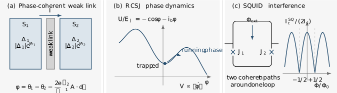
Three complementary Josephson descriptions. (a) A weak link couples two superconducting phases through the gauge-invariant difference $\phi$. (b) In the RCSJ analogy, current bias tilts the periodic Josephson energy; a trapped phase has zero mean voltage, while a running phase has $V\propto\langle\dot\phi\rangle$. (c) Two junctions in a loop form a dc SQUID whose critical current is flux periodic in the negligible-inductance, symmetric limit.

DC Josephson effect

For an ideal tunnel junction, the equilibrium supercurrent is

$$I_s(\phi) = I_c\sin\phi,$$

where $I_c>0$ is the critical current. A static phase can therefore support

$$\lvert I_s\rvert \le I_c$$

at zero junction voltage. The phrase DC Josephson effect refers to this stationary zero-voltage branch, not to a claim that every current-biased junction remains dissipationless for arbitrary current.

The corresponding coupling energy is

$$U_J(\phi) = -E_J\cos\phi,$$

with

$$E_J = \frac{\hbar I_c}{2e} = \frac{\Phi_0 I_c}{2\pi}.$$

Current follows from the phase derivative:

$$I_s = \frac{2e}{\hbar} \frac{\partial U_J}{\partial\phi} = \frac{2\pi}{\Phi_0} \frac{\partial U_J}{\partial\phi}.$$

This relation generalizes beyond a cosine. If the equilibrium junction free energy is $F_J(\phi)$, then

$$I_s(\phi) = \frac{2e}{\hbar} \frac{\partial F_J}{\partial\phi}.$$

A measured current–phase relation is therefore a derivative of the phase-dependent free energy, not merely a fitting curve.

Josephson inductance

For a small perturbation about a static operating point $\phi_0$,

$$\delta I = I_c\cos\phi_0\,\delta\phi.$$

Using the branch flux

$$\Phi_J \equiv \frac{\Phi_0}{2\pi}\phi,$$

the differential Josephson inductance is

$$L_J(\phi_0) \equiv \frac{\delta\Phi_J}{\delta I} = \frac{\Phi_0}{ 2\pi I_c\cos\phi_0 }.$$

It diverges at $\phi_0=\pi/2$ in the ideal sinusoidal model and changes sign beyond that point. A negative differential inductance is not by itself an unstable circuit; stability depends on the full network and bias condition.

Microscopic tunnel-junction scale

For identical isotropic BCS superconductors separated by a low-transparency insulating barrier, lowest-order tunneling theory gives the Ambegaokar–Baratoff relation

$$I_c(T)R_N = \frac{\pi\Delta(T)}{2e} \tanh\left[ \frac{\Delta(T)}{ 2k_{\mathrm B}T } \right],$$

where $R_N$ is the normal-state resistance and $\Delta(T)$ is the superconducting gap. At zero temperature,

$$I_cR_N = \frac{\pi\Delta_0}{2e}.$$

This product is a benchmark for an ideal symmetric SIS tunnel junction. It is not a universal law for:

• metallic or semiconductor weak links;
• high-transparency contacts;
• unequal or anisotropic gaps;
• strong pair breaking;
• multiband superconductors;
• unconventional order parameters;
• nonequilibrium quasiparticle distributions.

BCS Theory owns the gap equation, weak-coupling ratios, quasiparticle density of states, and tunneling convolution. The Josephson current is additionally phase sensitive: it depends on coherent anomalous amplitudes on both sides.

Beyond a sinusoidal current–phase relation

The most general $2\pi$-periodic relation can be expanded as

$$I(\phi) = \sum_{n=1}^{\infty} \left[ I_n^{(s)}\sin(n\phi) + I_n^{(c)}\cos(n\phi) \right].$$

If time-reversal and relevant spatial symmetries enforce

$$I(-\phi)=-I(\phi),$$

the cosine terms vanish. High transparency and long dwell times can generate substantial higher sine harmonics.

For one short spin-degenerate channel of transparency $\tau$ between equal $s$-wave gaps, the positive Andreev level is

$$E_A(\phi) = \Delta \sqrt{ 1-\tau\sin^2\left( \frac{\phi}{2} \right) }.$$

Its equilibrium contribution is

$$I_A(\phi) = \frac{ e\Delta^2 }{2\hbar} \frac{ \tau\sin\phi }{ E_A(\phi) } \tanh\left[ \frac{E_A(\phi)}{ 2k_{\mathrm B}T } \right].$$

For $\tau\ll1$, this reduces to a sinusoid. As $\tau$ approaches unity, the current becomes strongly nonsinusoidal. This microscopic expression assumes a short coherent contact and equilibrium level occupation; it is not a generic formula for every SNS junction.

Broken time-reversal and inversion symmetries can permit an anomalous phase shift,

$$I(\phi) = I_c\sin(\phi-\phi_0),$$

while a $\pi$ junction has its energy minimum near $\phi=\pi$. Such shifts require a stated microscopic mechanism; they should not be inferred from an arbitrary offset in an uncalibrated measurement.

AC Josephson effect

The second Josephson relation is

$$\dot\phi = \frac{2e}{\hbar}V = \frac{2\pi}{\Phi_0}V.$$

For constant voltage,

$$\phi(t) = \phi_0 + \frac{2eV}{\hbar}t,$$

so an ideal sinusoidal junction carries

$$I_s(t) = I_c \sin\left( \phi_0 + \frac{2eV}{\hbar}t \right).$$

The oscillation frequency is

$$f_J = \frac{2e}{h}\lvert V\rvert = K_J\lvert V\rvert,$$

where the Josephson constant is

$$K_J \equiv \frac{2e}{h} = 483\,597.848\,416\,984 \ \mathrm{GHz\,V^{-1}}$$

to the displayed BIPM value. Thus $1\ \mu\mathrm V$ corresponds to approximately $483.6\ \mathrm{MHz}$.

Because the revised SI fixes the numerical values of $e$ and $h$, the quotient $2e/h$ is exact in SI. Josephson voltage standards rely additionally on the experimentally established universality of the Josephson relation and on controlled phase locking in the device.

Shapiro steps

Drive the junction with angular frequency $\omega=2\pi f$. When the nonlinear phase dynamics locks so that

$$\left\langle \dot\phi \right\rangle = n\omega, \qquad n\in\mathbb Z,$$

the time-averaged voltage is quantized:

$$\langle V\rangle_n = n\frac{\hbar\omega}{2e} = n\frac{hf}{2e} = n\Phi_0 f.$$

These constant-voltage plateaus are Shapiro steps. In a simple overdamped sinusoidal model, their widths follow Bessel-function dependences on drive amplitude. Real step patterns also depend on capacitance, microwave coupling, impedance, heating, noise, higher harmonics, and spatial mode structure.

Fractional steps do not automatically prove fractional charge or topological superconductivity. Conventional higher harmonics and subharmonic locking can produce them. Conversely, a missing integer step is not by itself evidence for a protected $4\pi$-periodic mode: Landau–Zener transitions, quasiparticle poisoning, nonequilibrium occupations, and circuit dynamics can imitate that signature.

Magnetic interference across a junction

A magnetic field makes the gauge-invariant phase vary along an extended junction. For a short rectangular junction with uniform critical-current density and negligible self-field, integrating the local current gives

$$I_c(\Phi_J) = I_c(0) \left\lvert \frac{ \sin(\pi\Phi_J/\Phi_0) }{ \pi\Phi_J/\Phi_0 } \right\rvert.$$

This Fraunhofer-like pattern has ideal zeros at

$$\Phi_J = m\Phi_0, \qquad m\in\mathbb Z\setminus\{0\}.$$

Here $\Phi_J$ is the effective magnetic flux through the junction region, including penetration into the electrodes. It need not equal the applied field times the lithographic barrier area. Flux focusing, electrode screening, nonuniform current density, trapped vortices, faceting, self-fields, and finite junction length distort the pattern.

The inverse problem is informative but nonunique: a distorted $I_c(B)$ pattern constrains the spatial current distribution only after the electromagnetic geometry and phase retrieval assumptions are specified.

RCSJ dynamics and the electromagnetic environment

The resistively and capacitively shunted junction model places three elements in parallel:

1. an ideal Josephson element $I_c\sin\phi$;
2. a dissipative conductance $1/R$;
3. a capacitance $C$.

For current bias $I_b$,

$$I_b = I_c\sin\phi + \frac{V}{R} + C\dot V + I_{\mathrm n}(t).$$

Using $V=(\hbar/2e)\dot\phi$ gives

$$\frac{\hbar C}{2e} \ddot\phi + \frac{\hbar}{2eR} \dot\phi + I_c\sin\phi = I_b - I_{\mathrm n}(t),$$

where the sign assigned to the noise source follows the circuit convention.

The equation is analogous to a driven damped particle moving in the tilted washboard potential

$$U(\phi) = -E_J\cos\phi - \frac{\hbar I_b}{2e}\phi.$$

The dictionary is:

Junction quantity	Phase-particle analogue
capacitance $C$	inertia
conductance $1/R$	viscous damping
bias current $I_b$	constant tilt
Josephson energy $E_J$	periodic corrugation
voltage $V=(\hbar/2e)\dot\phi$	phase velocity
thermal or quantum noise	fluctuating force

For $\lvert I_b\rvert<I_c$, local minima exist. A phase trapped in a minimum has zero average voltage. Thermal activation or quantum tunneling can cause premature switching, so a measured switching current is generally a stochastic dynamical quantity rather than the equilibrium $I_c$ itself.

Characteristic scales

At zero bias, small oscillations have plasma frequency

$$\omega_{p0} = \sqrt{ \frac{2eI_c}{\hbar C} } = \frac{1}{ \sqrt{L_J(0)C} }.$$

At normalized bias $i_b=I_b/I_c$ with $\lvert i_b\rvert<1$,

$$\omega_p(i_b) = \omega_{p0} \left( 1-i_b^2 \right)^{1/4}.$$

Using the characteristic time

$$\tau = \omega_c t, \qquad \omega_c = \frac{2eI_cR}{\hbar},$$

the noiseless equation becomes

$$\beta_c \frac{d^2\phi}{d\tau^2} + \frac{d\phi}{d\tau} + \sin\phi = i_b,$$

where

$$\beta_c = \frac{2eI_cR^2C}{\hbar} = \frac{2\pi I_cR^2C}{\Phi_0}$$

is the Stewart–McCumber parameter. Roughly, $\beta_c\ll1$ is overdamped and $\beta_c\gg1$ is underdamped. Hysteresis also depends on frequency-dependent impedance, temperature, noise, and retrapping; one fitted $\beta_c$ is not a complete environmental model.

Overdamped current–voltage benchmark

For $C=0$, no noise, and $\lvert I_b\rvert>I_c$, the phase runs continuously. Averaging one $2\pi$ traversal gives

$$\langle V\rangle = R\, \operatorname{sgn}(I_b) \sqrt{ I_b^2-I_c^2 }.$$

Below $I_c$, the ideal deterministic model has a zero-voltage branch. Rounding near the transition can come from temperature, noise, inhomogeneity, frequency-dependent damping, or a distribution of junction parameters.

SQUID interference

A dc superconducting quantum interference device contains two Josephson junctions in a superconducting loop. Let the two phase differences be $\phi_1$ and $\phi_2$. Neglecting loop inductance, fluxoid consistency gives

$$\phi_1-\phi_2 = 2\pi \frac{\Phi_{\mathrm{ext}}}{\Phi_0} + 2\pi m, \qquad m\in\mathbb Z,$$

with a sign determined by loop orientation. For identical junctions,

$$\begin{aligned} I &= I_c\sin\phi_1 + I_c\sin\phi_2 \\ &= 2I_c \sin\bar\phi \cos\left( \pi\frac{\Phi_{\mathrm{ext}}}{\Phi_0} \right), \end{aligned}$$

where $\bar\phi=(\phi_1+\phi_2)/2$ after absorbing the integer winding. Maximizing over $\bar\phi$ gives

$$I_{c,\mathrm{SQUID}} \left( \Phi_{\mathrm{ext}} \right) = 2I_c \left\lvert \cos\left( \pi\frac{\Phi_{\mathrm{ext}}}{\Phi_0} \right) \right\rvert.$$

The modulation is periodic in $\Phi_0$. Junction asymmetry prevents complete cancellation at half-integer flux. Finite loop inductance makes the total flux

$$\Phi = \Phi_{\mathrm{ext}} + LI_{\mathrm{circ}},$$

so the circulating current and phases must be solved self-consistently. Flux noise, junction noise, readout backaction, trapped vortices, and the transfer function determine practical sensitivity.

A SQUID is therefore not simply “a detector of magnetic field.” It measures flux coupled into a calibrated loop and converts it through a nonlinear, bias-dependent transfer function.

Bridge to superconducting quantum circuits

Charge on a superconducting island and junction phase form a conjugate pair. With

$$[\phi,n]=i,$$

where $n$ counts excess Cooper pairs, a capacitively shunted junction has the elementary Hamiltonian

$$H = 4E_C(n-n_g)^2 - E_J\cos\phi, \qquad E_C = \frac{e^2}{2C_\Sigma}.$$

The quadratic expansion of the cosine supplies an inductive mode, while its higher powers supply anharmonicity:

$$-E_J\cos\phi = -E_J + \frac{E_J}{2}\phi^2 - \frac{E_J}{24}\phi^4 + \cdots.$$

This nonlinearity lets a circuit isolate two levels and operate as an artificial atom. Different devices trade charge sensitivity, flux sensitivity, anharmonicity, coupling, and control by choosing $E_J/E_C$, loop inductance, junction arrays, and bias points.

For two identical junctions in a negligible-inductance split loop,

$$H_J = -2E_{J0} \cos\left( \pi\frac{\Phi_{\mathrm{ext}}}{\Phi_0} \right) \cos\bar\phi.$$

External flux therefore tunes the signed effective Josephson coupling. Junction asymmetry rounds the nominal zero and modifies flux sensitivity.

This page stops at the physical junction and its elementary circuit degree of freedom. Circuit QED Overview owns transmon quantization, dispersive coupling, resonators, drive and readout Hamiltonians, coherence, and calibration.

Experimental inference workflow

1. Identify the junction class. Record materials, barrier or weak-link geometry, dimensions, interfaces, and whether transport is ballistic, diffusive, or tunneling.
2. Establish the superconducting state. Measure electrode gaps, transition temperatures, critical fields, and lead resistance independently.
3. Separate equilibrium and switching currents. Report current-ramp rate, filtering, temperature, switching distribution, and retrapping.
4. Measure the full current–voltage curve. Check zero-voltage, quasiparticle, excess-current, hysteretic, and heating regimes.
5. Resolve the current–phase relation when needed. A fitted $I_c$ alone cannot reveal higher harmonics or an anomalous phase shift.
6. Calibrate magnetic geometry. Include flux focusing, effective junction thickness, loop inductance, and trapped-flux history.
7. Test microwave locking. Verify that step voltages scale with frequency and integer index, and map widths versus drive power.
8. Model the environment. Infer impedance over the relevant frequency range rather than treating one DC resistance as universal.
9. Audit temperature and nonequilibrium. Electron heating and quasiparticle poisoning can dominate a nominally millikelvin experiment.
10. Cross-check microscopic scales. Compare $I_cR_N$, gap spectroscopy, channel transparency, normal conductance, and device dimensions.
11. Treat exotic signatures as composite claims. Rule out higher harmonics, Landau–Zener dynamics, poisoning, and inhomogeneity before assigning topological periodicity.

Common mistakes

Mistake	Why it fails	Better practice
Using $\theta_1-\theta_2$ as the observable phase in a field	The bare phase difference is gauge dependent	Include the line integral of $\mathbf A$
Calling Josephson current ordinary one-electron tunneling	It is coherent transfer tied to pair amplitudes on both sides	Distinguish supercurrent and quasiparticle current
Calling $I=I_c\sin\phi$ universal	Transparency, length, symmetry, and occupations alter the harmonics	Measure or calculate the current–phase relation
Equating switching current with $I_c$	Escape, noise, ramp rate, and heating shift switching	Report distributions and an environmental model
Treating $R$ in RCSJ as a universal material resistance	The relevant damping can be frequency dependent and nonlinear	Characterize the embedding impedance
Reading a Fraunhofer period from lithographic area alone	Screening and flux focusing change effective area	Calibrate geometry and field history
Calling every SQUID a field sensor	The loop responds to coupled flux through a transfer function	State effective area, inductance, bias, and noise
Interpreting fractional Shapiro steps as unique topology	Conventional harmonics and nonlinear locking also produce fractions	Test frequency, power, parity lifetime, and alternatives
Interpreting a missing first step as proof of $4\pi$ periodicity	Nonequilibrium and circuit dynamics can suppress steps	Combine independent phase-sensitive evidence
Using Ambegaokar–Baratoff for any weak link	It assumes a symmetric low-transparency SIS junction	Match the formula to the junction regime
Quantizing $-E_J\cos\phi$ without capacitance or constraints	A Hamiltonian needs conjugate charge and the full circuit graph	Derive $C_\Sigma$, offsets, loops, and modes
Treating gauge redundancy as a broken observable symmetry	Gauge-related phases describe the same physical state	Use phase differences, currents, fluxes, and response

Exercises

1. Verify gauge invariance

Show that

$$\phi = \theta_1-\theta_2 - \frac{2e}{\hbar} \int_1^2 \mathbf A\cdot d\boldsymbol{\ell}$$

is invariant under the gauge transformation stated in the convention ledger.

Solution

The electrode-phase contribution changes by

$$\delta(\theta_1-\theta_2) = -\frac{2e}{\hbar}\chi_1 + \frac{2e}{\hbar}\chi_2 = \frac{2e}{\hbar} (\chi_2-\chi_1).$$

The line integral changes by

$$\delta \int_1^2 \mathbf A\cdot d\boldsymbol{\ell} = \int_1^2 \boldsymbol{\nabla}\chi \cdot d\boldsymbol{\ell} = \chi_2-\chi_1.$$

Therefore

$$\delta\phi = \frac{2e}{\hbar} (\chi_2-\chi_1) - \frac{2e}{\hbar} (\chi_2-\chi_1) =0.$$

The cancellation is why magnetic interference can be expressed consistently in terms of phase.

2. Recover current and inductance from the energy

Starting from $U_J=-E_J\cos\phi$, derive the sinusoidal current and the differential inductance about $\phi_0$.

Solution

The phase derivative is

$$\frac{\partial U_J}{\partial\phi} = E_J\sin\phi.$$

Using $I=(2e/\hbar)\partial_\phi U_J$,

$$I = \frac{2eE_J}{\hbar}\sin\phi = I_c\sin\phi,$$

because $E_J=\hbar I_c/(2e)$.

Linearize around $\phi_0$:

$$\delta I = I_c\cos\phi_0\,\delta\phi.$$

Since $\delta\Phi_J=(\Phi_0/2\pi)\delta\phi$,

$$L_J(\phi_0) = \frac{\delta\Phi_J}{\delta I} = \frac{\Phi_0}{ 2\pi I_c\cos\phi_0 }.$$

3. Convert frequency to a Shapiro voltage

A junction is irradiated at $f=10.000\ \mathrm{GHz}$. Find the voltages of the $n=1$ and $n=5$ Shapiro steps.

Solution

The step voltage is

$$V_n = n\frac{f}{K_J} = n\Phi_0 f.$$

Using

$$K_J = 483\,597.848\,416\,984 \ \mathrm{GHz\,V^{-1}},$$

gives

$$V_1 \simeq 20.6783\ \mu\mathrm V,$$

and

$$V_5 \simeq 103.391\ \mu\mathrm V.$$

The integer spacing, not merely one plateau, is the robust phase-locking signature.

4. Use the Ambegaokar–Baratoff benchmark

An ideal symmetric SIS junction at low temperature has $\Delta_0=1.50\ \mathrm{meV}$ and $R_N=10.0\ \mathrm{k\Omega}$. Estimate $I_c$ and $E_J/k_{\mathrm B}$.

Solution

At $T=0$,

$$I_c = \frac{\pi\Delta_0}{2eR_N}.$$

Because $\Delta_0/e=1.50\ \mathrm{mV}$,

$$I_c = \frac{ \pi(1.50\ \mathrm{mV}) }{ 2(10.0\ \mathrm{k\Omega}) } \simeq 0.236\ \mu\mathrm A.$$

Then

$$\frac{E_J}{k_{\mathrm B}} = \frac{ \Phi_0I_c }{ 2\pi k_{\mathrm B} } \simeq 5.62\ \mathrm K.$$

Agreement with this estimate would support the SIS tunnel limit but would not independently prove all of its microscopic assumptions.

5. Infer an effective junction area

An ideal Fraunhofer pattern has adjacent zeros separated by $\Delta B=0.80\ \mathrm{mT}$. Neglecting field focusing, estimate the effective area.

Solution

Adjacent zeros differ by one flux quantum:

$$\Delta B\,A_{\mathrm{eff}} = \Phi_0.$$

Therefore

$$\begin{aligned} A_{\mathrm{eff}} &= \frac{ 2.068\times10^{-15}\ \mathrm{Wb} }{ 0.80\times10^{-3}\ \mathrm T } \\ &\simeq 2.58\times10^{-12}\ \mathrm{m^2} \\ &= 2.58\ \mu\mathrm m^2. \end{aligned}$$

This is a magnetic effective area. Comparing it with lithography requires penetration-depth and flux-focusing corrections.

6. Derive the symmetric SQUID envelope

For two identical junctions with negligible loop inductance, use

$$\phi_1-\phi_2 = 2\pi\frac{\Phi_{\mathrm{ext}}}{\Phi_0}$$

to derive the critical-current modulation.

Solution

Define

$$\bar\phi = \frac{\phi_1+\phi_2}{2}, \qquad \delta = \frac{\phi_1-\phi_2}{2} = \pi\frac{\Phi_{\mathrm{ext}}}{\Phi_0}.$$

The total current is

$$\begin{aligned} I &= I_c\sin(\bar\phi+\delta) + I_c\sin(\bar\phi-\delta) \\ &= 2I_c \sin\bar\phi \cos\delta. \end{aligned}$$

Maximizing its magnitude over $\bar\phi$ yields

$$I_{c,\mathrm{SQUID}} = 2I_c \left\lvert \cos\left( \pi\frac{\Phi_{\mathrm{ext}}}{\Phi_0} \right) \right\rvert.$$

Unequal junction critical currents leave a nonzero minimum at half-integer flux.

7. Derive the overdamped current–voltage curve

Set $C=0$ and noise to zero in the RCSJ equation. For $I_b>I_c$, average one $2\pi$ phase traversal to show that

$$\langle V\rangle = R\sqrt{I_b^2-I_c^2}.$$

Solution

The phase equation is

$$\frac{\hbar}{2eR}\dot\phi = I_b-I_c\sin\phi.$$

The traversal time is

$$\begin{aligned} T_\phi &= \frac{\hbar}{2eR} \int_0^{2\pi} \frac{d\phi}{ I_b-I_c\sin\phi } \\ &= \frac{\hbar}{2eR} \frac{2\pi}{ \sqrt{I_b^2-I_c^2} }. \end{aligned}$$

The mean phase velocity is $2\pi/T_\phi$, so

$$\begin{aligned} \langle V\rangle &= \frac{\hbar}{2e} \frac{2\pi}{T_\phi} \\ &= R\sqrt{I_b^2-I_c^2}. \end{aligned}$$

For negative bias, multiply by $\operatorname{sgn}(I_b)$. Noise rounds the ideal threshold.

8. Audit a missing Shapiro step claim

An experiment observes a suppressed $n=1$ step and claims a $4\pi$-periodic topological Josephson effect. Give a minimum evidence program that would make the claim substantially stronger.

Solution

A credible program should include:

1. map several integer and fractional steps versus microwave frequency and power;
2. fit a calibrated RCSJ or more complete environmental model including capacitance and frequency-dependent impedance;
3. test whether a conventional nonsinusoidal $2\pi$ current–phase relation reproduces the pattern;
4. quantify Landau–Zener transitions, heating, and nonequilibrium Andreev-level occupation;
5. measure quasiparticle-parity lifetime or poisoning rates;
6. reproduce the feature across devices, field orientations, gate settings, and sweep directions;
7. seek an independent phase-sensitive signature tied to the same topological regime;
8. verify the bulk or induced gap and rule out trivial subgap states.

A missing step is a useful anomaly, not a unique topological invariant.

Connections

• Unconventional Superconductivity uses phase-sensitive junction evidence to constrain gap sign and representation; this page retains current–phase laws, interference, voltage–frequency response, and the junction environment.
• London Theory owns gauge-invariant superflow, penetration, fluxoid quantization, and the electromagnetic origin of $\Phi_0$.
• Ginzburg–Landau Theory owns spatial order-parameter amplitude, critical fields, and vortex cores.
• Pair-Density Waves and Exotic Orders uses Josephson tunnelling as a momentum- and phase-sensitive diagnostic of finite-momentum pairing and higher-charge descendants.
• BCS Theory owns microscopic pairing, the superconducting gap, quasiparticles, and the tunnel-limit inputs to $I_cR_N$.
• Moiré Superconductivity uses gate-defined weak links, SQUID interference, and current–phase measurements as device-level tests of moiré coherence and pairing.
• Superconducting Proximity Effect determines equilibrium spatial pairing profiles, inverse suppression, and clean or diffusive weak-link scales before this page takes ownership of the gauge-invariant current–phase relation and phase dynamics.
• Proximity and Andreev Physics derives interface conversion, short-junction Andreev levels, and the transmission-resolved microscopic current carried by hybrid weak links.
• Tunneling Applications: First Encounters distinguishes coherent pair transfer from one-particle rectangular-barrier tunneling.
• Gauge Transformations in Quantum Mechanics supplies the phase and potential transformation rules.
• Off-Diagonal Long-Range Order gives number-conserving coherence diagnostics and explains why phase reference, gap, and stiffness are distinct.
• Periodic Hamiltonians supplies the language for driven phase locking beyond the elementary Shapiro result.
• Quantum Noise owns spectral conventions, quantum noise, and environmental backaction beyond a white-noise RCSJ source.
• Circuit QED Overview owns artificial-atom quantization, resonator coupling, dispersive readout, control, and device coherence.
• Superconducting Qubits carries junction and circuit physics into transmon and fluxonium processor architectures, local connectivity, packaging, and error-correction requirements.

References

1. B. D. Josephson, “Possible New Effects in Superconductive Tunnelling,” Physics Letters 1, 251–253 (1962), doi:10.1016/0031-9163(62)91369-0.
2. P. W. Anderson and J. M. Rowell, “Probable Observation of the Josephson Superconducting Tunneling Effect,” Physical Review Letters 10, 230–232 (1963), doi:10.1103/PhysRevLett.10.230.
3. V. Ambegaokar and A. Baratoff, “Tunneling Between Superconductors,” Physical Review Letters 10, 486–489 (1963), doi:10.1103/PhysRevLett.10.486; correction, Physical Review Letters 11, 104 (1963), doi:10.1103/PhysRevLett.11.104.
4. S. Shapiro, “Josephson Currents in Superconducting Tunneling: The Effect of Microwaves and Other Observations,” Physical Review Letters 11, 80–82 (1963), doi:10.1103/PhysRevLett.11.80.
5. R. C. Jaklevic, J. Lambe, A. H. Silver, and J. E. Mercereau, “Quantum Interference Effects in Josephson Tunneling,” Physical Review Letters 12, 159–160 (1964), doi:10.1103/PhysRevLett.12.159.
6. W. C. Stewart, “Current–Voltage Characteristics of Josephson Junctions,” Applied Physics Letters 12, 277–280 (1968), doi:10.1063/1.1651991.
7. D. E. McCumber, “Effect of ac Impedance on dc Voltage–Current Characteristics of Superconductor Weak-Link Junctions,” Journal of Applied Physics 39, 3113–3118 (1968), doi:10.1063/1.1656743.
8. K. K. Likharev, “Superconducting Weak Links,” Reviews of Modern Physics 51, 101–159 (1979), doi:10.1103/RevModPhys.51.101.
9. A. A. Golubov, M. Yu. Kupriyanov, and E. Il’ichev, “The Current–Phase Relation in Josephson Junctions,” Reviews of Modern Physics 76, 411–469 (2004), doi:10.1103/RevModPhys.76.411.
10. R. L. Kautz, “Noise, Chaos, and the Josephson Voltage Standard,” Reports on Progress in Physics 59, 935–992 (1996), doi:10.1088/0034-4885/59/8/001.
11. A. Barone and G. Paternò, Physics and Applications of the Josephson Effect, Wiley (1982), doi:10.1002/352760278X.
12. M. Tinkham, Introduction to Superconductivity, 2nd ed., Dover (2004).
13. J. Clarke and A. I. Braginski, eds., The SQUID Handbook, Volume 1: Fundamentals and Technology of SQUIDs and SQUID Systems, Wiley-VCH (2004), doi:10.1002/3527603646.
14. A. Blais, A. L. Grimsmo, S. M. Girvin, and A. Wallraff, “Circuit Quantum Electrodynamics,” Reviews of Modern Physics 93, 025005 (2021), doi:10.1103/RevModPhys.93.025005.
15. Bureau International des Poids et Mesures, “Practical realization of the volt,” SI Brochure, 9th ed., Appendix 2 (2019, updated), official BIPM appendix.