London Theory

London theory is the local, linear phenomenological electrodynamics of a superconductor with an established phase stiffness and nearly fixed condensate amplitude. It relates supercurrent to the gauge-invariant condensate momentum and predicts magnetic screening over the London penetration depth.

Its decisive achievement is not merely zero dc resistance. A perfect conductor can preserve whatever magnetic flux it started with. London theory instead describes an equilibrium state that expels magnetic field from the bulk, subject to geometry, topology, critical fields, and a finite surface layer. That is the Meissner response.

London theory does not explain why electrons pair, calculate the transition temperature, determine gap symmetry, resolve a vortex core, or decide whether a material is type I or type II. BCS Mean-Field Theory owns the microscopic paired saddle and quasiparticle spectrum. Off-Diagonal Long-Range Order owns the many-body coherence diagnostic. This page owns the macroscopic electromagnetic constitutive law and its experimentally testable consequences.

Use the Superfluidity and Superconductivity gateway when the claim may instead require Ginzburg–Landau, BCS, vortex, Josephson, proximity, or neutral-superfluid reasoning.

Required background. Classical Electromagnetism supplies Maxwell boundary-value problems, while Minimal Coupling in Wave Mechanics supplies the signed-charge gauge-covariant momentum used below.

Helpful background. Gauge Transformations in Quantum Mechanics fixes the phase and vector-potential bookkeeping, while Off-Diagonal Long-Range Order supplies a number-conserving coherence diagnostic.

Convention and density ledger

We use SI units and:

• $q^\ast$ for the signed charge of the coherent mobile object;
• $m^\ast$ for its effective inertial parameter;
• $n_s$ for its number density in the chosen convention;
• $\theta$ for the condensate phase;
• $\mathbf A$ for the vector potential, with $\mathbf B=\boldsymbol{\nabla}\times\mathbf A$;
• $\mathbf j_s$ for conventional electric current density;
• $\lambda_L$ for the local London penetration depth.

For Cooper pairs,

$$q^\ast=-2e, \qquad e>0.$$

If $n_s$ counts pairs, then $m^\ast$ and $q^\ast$ are pair parameters. Some texts instead count superconducting electrons and use an electron mass and charge magnitude. The combination entering electrodynamics is

$$\frac{n_s(q^\ast)^2}{m^\ast}.$$

Mixing a pair density with an electron mass or charge changes $\lambda_L$ by a spurious factor.

In a crystal, “$n_s/m^\ast$” is shorthand for a charge-stiffness tensor determined by bands, interactions, disorder, and temperature. It need not equal total carrier density divided by a free-electron mass. Penetration depth measures stiffness, not a literal head count of paired electrons without a model.

We distinguish:

• $\mathbf H_{\mathrm{appl}}$, controlled by external coils;
• $\mathbf B$, the local magnetic induction;
• $\mathbf H$, the auxiliary field inside a magnetized medium;
• demagnetizing fields set by sample shape.

London equations are local relations among $\mathbf j_s$, $\mathbf A$, and $\mathbf B$. Converting them into a measured magnetic moment requires Maxwell boundary conditions and geometry.

Gauge-invariant condensate momentum

Write a coarse-grained coherent field as

$$\Psi = \sqrt{n_s}\, e^{i\theta}.$$

Minimal coupling gives the mechanical momentum

$$\mathbf p_s = m^\ast\mathbf v_s = \hbar\boldsymbol{\nabla}\theta - q^\ast\mathbf A.$$

The supercurrent is

$$\mathbf j_s = n_sq^\ast\mathbf v_s = \frac{n_sq^\ast}{m^\ast} \left( \hbar\boldsymbol{\nabla}\theta - q^\ast\mathbf A \right).$$

Under a gauge transformation,

$$\mathbf A \longrightarrow \mathbf A+\boldsymbol{\nabla}\chi,$$

and

$$\theta \longrightarrow \theta + \frac{q^\ast}{\hbar}\chi.$$

Therefore

$$\hbar\boldsymbol{\nabla}\theta - q^\ast\mathbf A$$

is gauge invariant. The frequently quoted relation $\mathbf j_s\propto-\mathbf A$ is valid only after a phase and gauge choice in a simply connected region; it is not itself a gauge-invariant law.

A London free-energy functional with fixed $n_s$ is

$$\begin{aligned} F_L = \int\mathrm d^3r \bigg[ & \frac{n_s}{2m^\ast} \left| \hbar\boldsymbol{\nabla}\theta - q^\ast\mathbf A \right|^2 \\ & + \frac{|\mathbf B|^2}{2\mu_0} \bigg]. \end{aligned}$$

The electromagnetic convention is

$$\mathbf j_s = - \frac{\delta F_L}{ \delta\mathbf A }.$$

Varying the matter term therefore recovers the gauge-invariant current above. London screening is an equilibrium stiffness response, not an imposed rule that current must flow forever.

The London equations

The penetration depth is defined by

$$\lambda_L^2 = \frac{ m^\ast }{ \mu_0n_s(q^\ast)^2 }.$$

In the simplest uniform local model, the first London equation is

$$\frac{\partial\mathbf j_s}{\partial t} = \frac{ n_s(q^\ast)^2 }{ m^\ast } \mathbf E = \frac{1}{\mu_0\lambda_L^2} \mathbf E.$$

It describes reactive acceleration rather than Ohmic relaxation. By itself, it resembles ideal infinite conductivity and does not select an equilibrium magnetic field.

Taking the curl of the gauge-invariant current away from phase singularities gives the second London equation:

$$\boldsymbol{\nabla}\times\mathbf j_s = - \frac{ n_s(q^\ast)^2 }{ m^\ast } \mathbf B = - \frac{1}{\mu_0\lambda_L^2} \mathbf B.$$

This equation supplies the magnetic rigidity responsible for Meissner screening.

The split into “first” and “second” equations is historically useful but not fundamental. The phase-covariant current and an electromagnetic free energy make the assumptions clearer. Longitudinal electric response also requires charge conservation, scalar potential, compressibility, and phase dynamics; it is not fully described by the first equation in isolation.

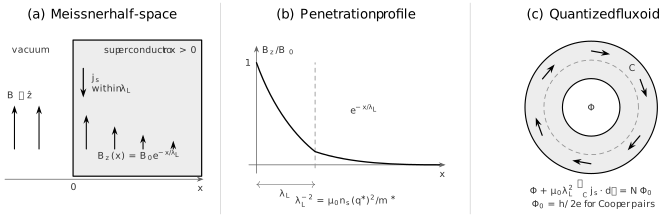
The London electrodynamics ledger. A surface current screens a static field from a superconducting half-space. The field decays as $e^{-x/\lambda_L}$ in the local model. In a multiply connected ring, phase winding quantizes the fluxoid $\Phi+\mu_0\lambda_L^2\oint\mathbf j_s\cdot\mathrm d\boldsymbol{\ell}$; magnetic flux alone is only approximately quantized when the contour current is negligible.

Meissner screening

In magnetostatics and away from external current leads,

$$\boldsymbol{\nabla}\times\mathbf B = \mu_0\mathbf j_s.$$

Take a curl:

$$\boldsymbol{\nabla}\times \left( \boldsymbol{\nabla}\times\mathbf B \right) = \mu_0 \boldsymbol{\nabla}\times\mathbf j_s.$$

Using

$$\boldsymbol{\nabla}\cdot\mathbf B=0$$

and the second London equation gives

$$\nabla^2\mathbf B = \frac{\mathbf B}{\lambda_L^2}.$$

This has exponentially decaying, rather than oscillatory, solutions.

Half-space

Let a superconductor occupy $x>0$, with a static field parallel to its surface:

$$\mathbf B(x) = B_z(x)\hat{\mathbf z}.$$

The bounded solution is

$$B_z(x) = B_0e^{-x/\lambda_L}.$$

Ampère’s law gives

$$j_{s,y}(x) = - \frac{1}{\mu_0} \frac{\mathrm dB_z}{\mathrm dx} = \frac{B_0}{\mu_0\lambda_L} e^{-x/\lambda_L}$$

for this orientation. The integrated sheet current is

$$K_y = \int_0^\infty j_{s,y}(x)\,\mathrm dx = \frac{B_0}{\mu_0}.$$

Thus the apparently sharp surface current of elementary magnetostatics is actually distributed over a layer of thickness $\lambda_L$.

The magnetic and condensate kinetic energy densities are

$$u_B = \frac{B^2}{2\mu_0},$$

and

$$u_{\mathrm{kin}} = \frac{m^\ast j_s^2}{ 2n_s(q^\ast)^2 } = \frac{\mu_0\lambda_L^2j_s^2}{2}.$$

For the ideal half-space solution,

$$u_{\mathrm{kin}}=u_B$$

point by point. Screening stores energy in both the field and coherent flow.

A finite slab

For a slab of thickness $d$ occupying

$$-\frac d2 \le x\le \frac d2,$$

with equal parallel field $B_a$ at both faces, symmetry gives

$$B_z(x) = B_a \frac{ \cosh(x/\lambda_L) }{ \cosh[d/(2\lambda_L)] }.$$

The spatial average is

$$\langle B_z\rangle = B_a \frac{ 2\lambda_L }{ d } \tanh \left( \frac{d}{2\lambda_L} \right).$$

For $d\gg\lambda_L$, most of the slab is field free. For $d\ll\lambda_L$, the field penetrates nearly uniformly and the bulk exponential picture is a poor visual approximation.

Meissner state versus perfect conductivity

Suppose an ordinary conductor somehow acquired exactly zero resistivity. Ohm’s law and Faraday’s law would imply that magnetic flux cannot change after the zero-resistance state is reached:

$$\frac{\partial\mathbf B}{\partial t} = 0$$

in the idealized bulk. The final field would depend on preparation history.

A superconductor in the equilibrium Meissner state instead selects a screened field configuration whether it is cooled before or after a weak field is applied, provided the same equilibrium phase is reached and flux is not trapped behind barriers. The second London equation encodes this distinction.

Real samples can trap flux because of vortices, defects, geometric barriers, metastability, or incomplete equilibration. Observing remanent field does not repeal the Meissner effect; it means the experiment is not sampling an ideal reversible Meissner state.

Zero resistance is a transport statement. Meissner screening is an equilibrium transverse response. Pair binding, a spectral gap, phase stiffness, and magnetic flux expulsion are related in a superconductor but remain distinct diagnostics.

Penetration depth as a material observable

The local London relation implies

$$\lambda_L^{-2} \propto \frac{n_s}{m^\ast}.$$

A common normalized superfluid-stiffness proxy is

$$\rho_s(T) \equiv \frac{ \lambda_L^2(0) }{ \lambda_L^2(T) }.$$

In a clean, local, isotropic, fully gapped weak-coupling benchmark at low temperature,

$$\frac{ \Delta\lambda_L(T) }{ \lambda_L(0) } \simeq \sqrt{ \frac{ \pi\Delta_0 }{ 2k_{\mathrm B}T } } \exp \left( - \frac{\Delta_0}{ k_{\mathrm B}T } \right).$$

Line nodes often produce a leading linear-$T$ correction in the clean local limit, while point nodes can produce a quadratic correction. Disorder, nonlocality, multiple gaps, surface states, magnetic impurities, and dimensional crossover can change these powers. Penetration-depth data constrain a gap model only after those alternatives and the measurement geometry are addressed.

Anisotropic stiffness

For a crystalline material, write

$$j_{s,i} = n_sq^\ast \left( \mathsf M^{-1} \right)_{ij} \left( \hbar\partial_j\theta - q^\ast A_j \right).$$

The inverse squared penetration-depth tensor is

$$\left( \mathsf\Lambda^{-2} \right)_{ij} = \mu_0n_s(q^\ast)^2 \left( \mathsf M^{-1} \right)_{ij}.$$

Crystal axes, field orientation, sample shape, and current direction must accompany a quoted $\lambda$. In multiband materials, stiffnesses from different bands add at the response-kernel level; one scalar “effective mass” may hide the relevant physics.

Experimental routes

Penetration depth can be inferred using:

• microwave cavity and surface-impedance measurements;
• tunnel-diode resonators;
• two-coil mutual inductance in films;
• muon spin rotation in appropriate field geometries;
• low-energy muons or depth-resolved magnetic probes;
• magnetic force, scanning SQUID, or NV measurements with a forward field model.

Many techniques measure

$$\Delta\lambda(T) = \lambda(T)-\lambda(T_{\mathrm{base}})$$

more accurately than the absolute $\lambda(0)$. Demagnetization, surface roughness, calibration standards, normal-fluid conductivity, vortex entry, and sample dimensions can dominate systematic uncertainty.

Fluxoid quantization preview

Single-valuedness of the coherent field requires

$$\oint_{\mathcal C} \boldsymbol{\nabla}\theta\cdot \mathrm d\boldsymbol{\ell} = 2\pi N, \qquad N\in\mathbb Z,$$

for a closed contour $\mathcal C$ that remains in a region where $\Psi\ne0$.

From

$$m^\ast\mathbf v_s + q^\ast\mathbf A = \hbar\boldsymbol{\nabla}\theta,$$

integration gives

$$m^\ast \oint_{\mathcal C} \mathbf v_s\cdot \mathrm d\boldsymbol{\ell} + q^\ast\Phi = Nh,$$

where

$$\Phi = \oint_{\mathcal C} \mathbf A\cdot \mathrm d\boldsymbol{\ell} = \int_{\mathcal S} \mathbf B\cdot\mathrm d\mathbf S.$$

Using $\mathbf j_s=n_sq^\ast\mathbf v_s$ and the London definition of $\lambda_L$,

$$\Phi + \mu_0\lambda_L^2 \oint_{\mathcal C} \mathbf j_s\cdot \mathrm d\boldsymbol{\ell} = N\frac{h}{q^\ast}.$$

The left-hand side is the fluxoid. Absorbing orientation and the sign of $q^\ast$ into the integer, its quantum has magnitude

$$\Phi_0 = \frac{h}{|q^\ast|}.$$

For Cooper pairs,

$$\Phi_0 = \frac{h}{2e} \simeq 2.068\times10^{-15}\, \mathrm{Wb}.$$

In a thick superconducting ring, choose $\mathcal C$ deep enough that $\mathbf j_s$ is negligible. Then

$$\Phi \simeq N\Phi_0.$$

In a thin wall or near a current-carrying surface, the current term need not vanish. The fluxoid is quantized; enclosed magnetic flux need not be exactly an integer multiple of $\Phi_0$.

In a simply connected, nonsingular Meissner region, a loop can shrink to a point and $N=0$. Nonzero winding requires a hole, a vortex core where the amplitude is suppressed, or another excluded region. London theory describes currents outside a vortex core but cannot resolve the core itself.

Thin films and the Pearl scale

For a film of thickness

$$d\ll\lambda_L,$$

current is nearly uniform across the thickness, but the magnetic field spreads far through the surrounding vacuum. Using the convention adopted here, the Pearl screening length is

$$\Lambda_P = \frac{ 2\lambda_L^2 }{ d }.$$

Some authors define $\lambda_L^2/d$ and call that quantity the Pearl length. The factor-of-two convention must be stated.

At distances below and above $\Lambda_P$, vortex currents and interactions have different spatial forms from bulk Abrikosov vortices. A thin film can therefore have $d\ll\lambda_L$ while magnetic screening remains important over a much larger in-plane distance.

Frequency-domain response

With time dependence $e^{-i\omega t}$, the first London equation gives

$$\mathbf j_s(\omega) = \sigma_s(\omega) \mathbf E(\omega),$$

where

$$\sigma_s(\omega) = \frac{i}{ \mu_0\omega\lambda_L^2 }.$$

The inductive $1/\omega$ imaginary conductivity is accompanied, by causality, by a zero-frequency delta function in the ideal real conductivity. At nonzero temperature and frequency, quasiparticles add dissipative conductivity. Terahertz and Infrared Probes develops how this complex response is measured, including gap thresholds, missing-area tests, substrates, and phase errors. Coherence factors, impurities, strong coupling, and collective modes lie beyond the lossless London kernel.

Penetration of an ac field is generally complex. With the $e^{-i\omega t}$ convention, one may write

$$\widetilde\lambda(\omega) = \lambda_1(\omega) - i\lambda_2(\omega),$$

or equivalently described through surface impedance. A measured microwave penetration depth is not automatically the static $\lambda_L$.

Locality and limits

London theory assumes a local constitutive relation:

$$\mathbf j_s(\mathbf r) \quad \text{depends on} \quad \mathbf A(\mathbf r) \ \text{and}\ \boldsymbol{\nabla}\theta(\mathbf r).$$

In a clean superconductor whose coherence scale is not small relative to the field-variation scale, response can be nonlocal. A gauge-invariant schematic form is

$$j_i(\mathbf r) = \int \mathcal K_{ij}(\mathbf r,\mathbf r') \left[ \hbar\partial_j'\theta(\mathbf r') - q^\ast A_j(\mathbf r') \right] \mathrm d^3r'.$$

This is the Pippard regime. The local London limit is recovered when the kernel is short ranged compared with the electromagnetic variation.

London theory also assumes:

• nearly fixed condensate amplitude;
• weak fields and currents relative to depairing scales;
• no explicit vortex-core structure;
• a local linear response kernel;
• sufficiently slow variation for a continuum description;
• negligible normal-fluid dissipation in its simplest form;
• known geometry and boundary conditions.

It cannot determine:

• the pairing mechanism or $T_c$;
• superconducting gap magnitude or symmetry;
• coherence length from amplitude healing;
• thermodynamic critical field;
• type-I versus type-II boundary;
• lower and upper critical fields;
• vortex-core energy;
• nonlinear critical current;
• surface pair breaking or proximity structure.

Those omissions are not defects in a phenomenological theory; they define its domain.

Experimental inference workflow

1. Declare geometry. Give field orientation, current path, dimensions, and demagnetizing factor.
2. Identify the electromagnetic regime. Distinguish static Meissner, mixed state, critical state, microwave, and transport conditions.
3. Compare every dimension with $\lambda$. Bulk, slab, film, wire, and ring formulas are not interchangeable.
4. Check vortex exclusion. Field cooling, trapped flux, edge barriers, and pinning can dominate apparent screening.
5. Separate absolute and relative calibration. $\Delta\lambda(T)$ and $\lambda(0)$ often have different uncertainties.
6. Test locality and anisotropy. Mean free path, coherence scale, crystal orientation, and multiband response matter.
7. Propagate backgrounds. Sample holder, substrate, normal-fluid loss, paramagnetic impurities, and surface layers can mimic low-temperature power laws.
8. Use orthogonal observables. Heat capacity, spectroscopy, critical fields, and phase-sensitive probes test interpretations that $\lambda(T)$ alone cannot settle.

Common mistakes

Mistake	Why it fails	Better practice
Equating zero resistance with the Meissner effect	A perfect conductor can freeze arbitrary initial flux	Compare equilibrium cooling and field histories
Writing $\mathbf j_s\propto-\mathbf A$ as a physical law	$\mathbf A$ is gauge dependent	Use $\hbar\nabla\theta-q^\ast\mathbf A$
Mixing pair and electron densities	$n_s$, $q^\ast$, and $m^\ast$ must share one convention	Report the full stiffness combination
Saying the bulk field is exactly zero everywhere	Field penetrates over $\lambda_L$ and depends on geometry	Solve the boundary-value problem
Calling flux exactly quantized in every ring	The current term quantizes the fluxoid	State when the contour current is negligible
Using a bulk $\lambda$ formula for a thin film	Stray fields spread over the Pearl scale	Compare $d$, $\lambda_L$, and lateral dimensions
Reading gap symmetry from one power law	Disorder, nonlocality, multiple gaps, and surfaces alter $\Delta\lambda$	Combine temperature, field, orientation, and other probes
Using London theory inside a vortex core	The fixed-amplitude assumption fails	Use an amplitude-resolving theory
Treating $n_s/m^\ast$ as total density over bare mass	Lattice and interaction effects renormalize stiffness	Interpret the response tensor microscopically
Ignoring trapped vortices in a penetration experiment	Vortex motion adds screening and dissipation	Establish the Meissner regime and field history

Exercises

1. Gauge invariance of the current

Show that

$$\mathbf j_s = \frac{n_sq^\ast}{m^\ast} \left( \hbar\boldsymbol{\nabla}\theta - q^\ast\mathbf A \right)$$

is invariant under the gauge transformation stated above.

Solution

The transformed combination is

$$\begin{aligned} \hbar\boldsymbol{\nabla}\theta' - q^\ast\mathbf A' &= \hbar\boldsymbol{\nabla} \left( \theta+\frac{q^\ast}{\hbar}\chi \right) \\ &\quad - q^\ast \left( \mathbf A+\boldsymbol{\nabla}\chi \right) \\ &= \hbar\boldsymbol{\nabla}\theta + q^\ast\boldsymbol{\nabla}\chi - q^\ast\mathbf A - q^\ast\boldsymbol{\nabla}\chi \\ &= \hbar\boldsymbol{\nabla}\theta - q^\ast\mathbf A. \end{aligned}$$

Therefore $\mathbf j_s$ is invariant. The phase and vector potential separately depend on gauge; their covariant combination does not.

2. Derive the screening equation

Starting from magnetostatic Ampère law and the second London equation, derive the differential equation for $\mathbf B$.

Solution

Take the curl of

$$\boldsymbol{\nabla}\times\mathbf B = \mu_0\mathbf j_s:$$ $$\boldsymbol{\nabla}\times \left( \boldsymbol{\nabla}\times\mathbf B \right) = \mu_0 \boldsymbol{\nabla}\times\mathbf j_s.$$

The vector identity and $\boldsymbol{\nabla}\cdot\mathbf B=0$ give

$$\boldsymbol{\nabla}\times \left( \boldsymbol{\nabla}\times\mathbf B \right) = - \nabla^2\mathbf B.$$

The second London equation gives

$$\mu_0 \boldsymbol{\nabla}\times\mathbf j_s = - \frac{\mathbf B}{\lambda_L^2}.$$

Hence

$$\nabla^2\mathbf B = \frac{\mathbf B}{\lambda_L^2}.$$

3. Half-space sheet current

For $B_z(x)=B_0e^{-x/\lambda_L}$ in $x>0$, find $j_y(x)$ and its integral over depth.

Solution

For $\mathbf B=B_z(x)\hat{\mathbf z}$,

$$\left( \boldsymbol{\nabla}\times\mathbf B \right)_y = - \frac{\mathrm dB_z}{\mathrm dx}.$$

Thus

$$j_y(x) = - \frac{1}{\mu_0} \frac{\mathrm dB_z}{\mathrm dx} = \frac{B_0}{\mu_0\lambda_L} e^{-x/\lambda_L}.$$

The sheet current is

$$\begin{aligned} K_y &= \int_0^\infty j_y(x)\,\mathrm dx \\ &= \frac{B_0}{\mu_0\lambda_L} \int_0^\infty e^{-x/\lambda_L}\,\mathrm dx \\ &= \frac{B_0}{\mu_0}. \end{aligned}$$

Its sign reverses if the surface normal or applied field reverses.

4. Field in a symmetric slab

Solve

$$\frac{\mathrm d^2B}{\mathrm dx^2} = \frac{B}{\lambda_L^2}$$

for a slab with $B(\pm d/2)=B_a$. Check the thick- and thin-slab limits of the central field.

Solution

The general solution is

$$B(x) = C\cosh(x/\lambda_L) + D\sinh(x/\lambda_L).$$

Equal boundary values and reflection symmetry require $D=0$. Imposing either face gives

$$B(x) = B_a \frac{ \cosh(x/\lambda_L) }{ \cosh[d/(2\lambda_L)] }.$$

At the center,

$$B(0) = \frac{B_a}{ \cosh[d/(2\lambda_L)] }.$$

For $d\gg\lambda_L$,

$$B(0)\to0.$$

For $d\ll\lambda_L$,

$$\cosh[d/(2\lambda_L)] \simeq1,$$

so $B(0)\simeq B_a$: a very thin slab cannot exclude a parallel field from most of its thickness.

5. Fluxoid rather than flux

Derive fluxoid quantization from phase winding. Under what condition does it reduce to flux quantization?

Solution

Integrate

$$m^\ast\mathbf v_s + q^\ast\mathbf A = \hbar\boldsymbol{\nabla}\theta$$

around a closed contour:

$$m^\ast \oint\mathbf v_s\cdot\mathrm d\boldsymbol{\ell} + q^\ast\Phi = \hbar(2\pi N) = Nh.$$

Because

$$\mathbf v_s = \frac{\mathbf j_s}{n_sq^\ast}$$

and

$$\frac{m^\ast}{ n_s(q^\ast)^2 } = \mu_0\lambda_L^2,$$

division by $q^\ast$ gives

$$\Phi + \mu_0\lambda_L^2 \oint \mathbf j_s\cdot\mathrm d\boldsymbol{\ell} = N\frac{h}{q^\ast}.$$

If the contour lies deep inside a thick superconducting wall where $\mathbf j_s\simeq0$, then the magnetic flux itself is approximately quantized in units $h/|q^\ast|$.

6. Inductive conductivity

Using $e^{-i\omega t}$ time dependence, derive the London conductivity and identify its phase relative to the electric field.

Solution

The first London equation becomes

$$-i\omega\mathbf j_s = \frac{\mathbf E}{ \mu_0\lambda_L^2 }.$$

Therefore

$$\mathbf j_s = \frac{i}{ \mu_0\omega\lambda_L^2 } \mathbf E,$$

so

$$\sigma_s(\omega) = \frac{i}{ \mu_0\omega\lambda_L^2 }.$$

The current is $90^\circ$ out of phase with the field in this lossless convention. A real material also has dissipative quasiparticle and vortex contributions.

7. Pearl scale and conventions

A film has $d=20\,\mathrm{nm}$ and $\lambda_L=200\,\mathrm{nm}$. Find $\Lambda_P=2\lambda_L^2/d$. Why must a reported “Pearl length” include its definition?

Solution

Using consistent units,

$$\Lambda_P = \frac{ 2(200\,\mathrm{nm})^2 }{ 20\,\mathrm{nm} } = 4000\,\mathrm{nm} = 4.0\,\mu\mathrm m.$$

The in-plane screening scale is much larger than either $d$ or $\lambda_L$. Some authors define the Pearl length as $\lambda_L^2/d$, which would give $2.0\,\mu\mathrm m$ for the same film. The physics is unchanged, but an unlabeled numerical value is ambiguous by a factor of two.

Connections

• Unconventional Superconductivity treats penetration-depth anisotropy and low-temperature behavior as one constraint in a multi-probe gap-symmetry audit; this page retains the electrodynamic kernel, geometry, and inversion limits.
• Classical Electromagnetism Before Quantum Theory supplies Maxwell equations, induction, and constitutive-field conventions.
• Minimal Coupling in Wave Mechanics develops $\mathbf p-q\mathbf A$ for a charged quantum particle.
• Ginzburg–Landau Theory lets the superconducting amplitude vary and owns coherence length, critical scales, type-I/type-II behavior, and vortex cores.
• Vortex Matter, Pinning, and Flux Flow begins outside the static core solution and owns collective interactions, pinning, creep, and driven flux motion rather than London electrodynamics.
• Gauge Transformations in Quantum Mechanics owns the wavefunction and potential transformation rules.
• Off-Diagonal Long-Range Order distinguishes coherence from stiffness, pair binding, a spectral gap, and Meissner response.
• Order Parameters gives the source-selected and response-aware language for ordered phases.
• BCS Theory connects microscopic pairing, quasiparticle thermodynamics, and the long-wavelength electromagnetic stiffness used here.
• Josephson Effect turns gauge-invariant phase differences into current, voltage–frequency locking, and SQUID flux interference.
• BCS Mean-Field Theory develops the reduced Hamiltonian, paired saddle, gap equation, and Bogoliubov quasiparticles.
• Susceptibilities develops response kernels, longitudinal versus transverse limits, and internal-field corrections.
• From Phase Symmetry to Gauge Theory explains why a gauge redundancy is not itself an observable broken global symmetry.
• What Is Quantum Matter? places Meissner response and phase stiffness among the defining diagnostics of superconductivity.

References

1. W. Meissner and R. Ochsenfeld, “Ein neuer Effekt bei Eintritt der Supraleitfähigkeit,” Die Naturwissenschaften 21, 787–788 (1933), doi:10.1007/BF01504252.
2. F. London and H. London, “The electromagnetic equations of the supraconductor,” Proceedings of the Royal Society A 149, 71–88 (1935), doi:10.1098/rspa.1935.0048.
3. F. London, Superfluids, Volume I: Macroscopic Theory of Superconductivity, 2nd ed., Dover (1961).
4. M. Tinkham, Introduction to Superconductivity, 2nd ed., Dover (2004).
5. P. G. de Gennes, Superconductivity of Metals and Alloys, Westview Press (1999).
6. D. Shoenberg, Superconductivity, 2nd ed., Cambridge University Press (1952).
7. A. B. Pippard, “An experimental and theoretical study of the relation between magnetic field and current in a superconductor,” Proceedings of the Royal Society A 216, 547–568 (1953), doi:10.1098/rspa.1953.0040.
8. B. S. Deaver, Jr. and W. M. Fairbank, “Experimental evidence for quantized flux in superconducting cylinders,” Physical Review Letters 7, 43–46 (1961), doi:10.1103/PhysRevLett.7.43.
9. R. Doll and M. Näbauer, “Experimental proof of magnetic flux quantization in a superconducting ring,” Physical Review Letters 7, 51–52 (1961), doi:10.1103/PhysRevLett.7.51.
10. J. Pearl, “Current distribution in superconducting films carrying quantized fluxoids,” Applied Physics Letters 5, 65–66 (1964), doi:10.1063/1.1754056.
11. P. W. Anderson, “Plasmons, gauge invariance, and mass,” Physical Review 130, 439–442 (1963), doi:10.1103/PhysRev.130.439.
12. R. Prozorov and R. W. Giannetta, “Magnetic penetration depth in unconventional superconductors,” Superconductor Science and Technology 19, R41–R67 (2006), doi:10.1088/0953-2048/19/8/R01.
13. W. N. Hardy, D. A. Bonn, D. C. Morgan, R. Liang, and K. Zhang, “Precision measurements of the temperature dependence of $\lambda$ in $\mathrm{YBa_2Cu_3O_{6.95}}$: Strong evidence for nodes in the gap function,” Physical Review Letters 70, 3999–4002 (1993), doi:10.1103/PhysRevLett.70.3999.
14. P. J. Hirschfeld and N. Goldenfeld, “Effect of strong scattering on the low-temperature penetration depth of a $d$-wave superconductor,” Physical Review B 48, 4219–4222 (1993), doi:10.1103/PhysRevB.48.4219.
15. J. Bardeen, L. N. Cooper, and J. R. Schrieffer, “Theory of superconductivity,” Physical Review 108, 1175–1204 (1957), doi:10.1103/PhysRev.108.1175.