Ginzburg–Landau Theory

Ginzburg–Landau theory is the static, gauge-covariant effective theory of a superconducting order parameter that may vary in space. It extends London Theory by allowing the condensate amplitude to heal, vanish at boundaries and vortex cores, and respond nonlinearly to magnetic field and current.

The theory is phenomenological in the precise sense that symmetry and locality determine the form of the free energy, while experiment or a microscopic calculation determines its coefficients. Near a continuous superconducting transition, that separation is powerful enough to predict two material lengths, magnetic critical scales, the type-I/type-II criterion, flux-carrying vortices, and characteristic temperature dependences.

This page owns the material phenomenology of the single-component local theory. Landau–Ginzburg Theory Preview owns the generic coarse-grained field, Gaussian correlation length, interfaces, fluctuations, and Ginzburg criterion. BCS Mean-Field Theory owns the microscopic paired saddle and gap equation. Full critical field theory and renormalization belong to the field-theory continuation.

Use the Superfluidity and Superconductivity gateway when the question instead concerns fixed-amplitude electrodynamics, microscopic pairing, vortex motion, weak links, proximity, or unconventional evidence.

Required background. London Theory supplies the fixed-amplitude electromagnetic limit, while Landau–Ginzburg Theory Preview supplies the coarse-grained functional, stability, correlation-length, and fluctuation language used here.

Helpful background. Order Parameters supplies normalization and symmetry discipline, while Minimal Coupling in Wave Mechanics supplies the gauge-covariant gradient construction.

Scope and convention ledger

We use SI units and the free-energy density convention

$$f_{\mathrm{pot}} = \alpha|\psi|^2 + \frac{\beta}{2}|\psi|^4.$$

The symbols mean:

• $\psi(\mathbf r)$ is a coarse-grained complex superconducting order parameter;
• $q^\ast$ is the signed charge carried by the coherent field;
• $m^\ast$ is the mass parameter in the gradient term;
• $\alpha$ and $\beta$ are phenomenological coefficients;
• $\mathbf A$ is the vector potential and $\mathbf B=\boldsymbol{\nabla}\times\mathbf A$;
• $\mu_0$ is the vacuum permeability;
• $\Phi_0=h/|q^\ast|$ is the flux quantum.

For an ordinary Cooper-pair condensate,

$$q^\ast=-2e, \qquad \Phi_0=\frac{h}{2e}.$$

We choose the convenient normalization

$$|\psi|^2=n_s,$$

so $|\psi|^2$ has the dimensions of a pair density and the gradient coefficient is written with $m^\ast$. This normalization is not universal. A rescaling

$$\psi\longrightarrow c\psi$$

reshuffles $\alpha$, $\beta$, and the gradient coefficient without changing observables. A quoted GL coefficient has meaning only together with the order-parameter normalization.

Near a mean-field transition,

$$\alpha(T) = \alpha_0(T-T_c), \qquad \alpha_0>0, \qquad \beta>0,$$

while $\beta$ and $m^\ast$ are often approximated as smooth constants. This linear form is an asymptotic expansion near $T_c$, not a global law down to zero temperature.

The magnetic thermodynamic ensemble also matters. The functional below includes the internal field energy and is convenient when fields and boundary conditions are solved together. At fixed applied field, equilibrium comparison requires the appropriate Gibbs potential and the energy of the external-field apparatus. One must distinguish:

$$\mathbf H_{\mathrm{appl}}, \qquad \mathbf H, \qquad \mathbf B,$$

and include demagnetizing fields before comparing a bulk formula with a measured magnetization.

Order parameter and uniform equilibrium

Write

$$\psi(\mathbf r) = |\psi(\mathbf r)|e^{i\theta(\mathbf r)}.$$

Under the electromagnetic gauge transformation

$$\begin{aligned} \mathbf A &\longrightarrow \mathbf A+\boldsymbol{\nabla}\chi, \\ \theta &\longrightarrow \theta+\frac{q^\ast}{\hbar}\chi, \end{aligned}$$

the order parameter transforms as

$$\psi \longrightarrow e^{iq^\ast\chi/\hbar}\psi.$$

The phase by itself is gauge dependent. Gauge-invariant information resides in $|\psi|$, magnetic field, current, phase winding around a closed contour, and the covariant phase gradient

$$\hbar\boldsymbol{\nabla}\theta - q^\ast\mathbf A.$$

The GL order parameter is not a literal two-electron Schrödinger wavefunction. It is a coarse-grained collective field whose normalization and microscopic relation depend on the derivation. Off-Diagonal Long-Range Order supplies the number-conserving many-body coherence diagnostic.

Uniform minimum

With no field, current, or spatial variation, minimize

$$f_{\mathrm{pot}}(u) = \alpha u + \frac{\beta}{2}u^2, \qquad u=|\psi|^2.$$

The stationary solutions satisfy

$$\psi \left( \alpha+\beta|\psi|^2 \right) =0.$$

For $\alpha>0$, the stable minimum is

$$\psi_\infty=0.$$

For $\alpha<0$,

$$|\psi_\infty|^2 = - \frac{\alpha}{\beta}.$$

The phase is undetermined until gradients, boundaries, or external couplings are specified. The condensation free-energy density relative to the normal state is

$$\Delta f_{\mathrm{cond}} = f_s-f_n = - \frac{\alpha^2}{2\beta}.$$

Equating its magnitude to the magnetic energy density defines the thermodynamic critical induction $B_c$:

$$\frac{B_c^2}{2\mu_0} = \frac{\alpha^2}{2\beta},$$

so

$$B_c = |\alpha| \sqrt{\frac{\mu_0}{\beta}}.$$

This is a bulk thermodynamic scale. An observed entry or exit field can differ because of surface barriers, pinning, geometry, metastability, or type-II vortex physics.

Gauge-covariant free energy

Define the mechanical-momentum operator

$$\boldsymbol{\Pi} = - i\hbar\boldsymbol{\nabla} - q^\ast\mathbf A.$$

The minimal isotropic single-component functional is

$$\begin{aligned} F_{\mathrm{GL}}[\psi,\mathbf A] = \int_\Omega\mathrm d^3r \bigg[ & \alpha|\psi|^2 + \frac{\beta}{2}|\psi|^4 \\ & + \frac{1}{2m^\ast} \left| \boldsymbol{\Pi}\psi \right|^2 + \frac{|\mathbf B|^2}{2\mu_0} \bigg]. \end{aligned}$$

Each term has a distinct role:

Term	Physical content	What fixes its coefficient
$\alpha\lvert\psi\rvert^2+\beta\lvert\psi\rvert^4/2$	local preference for normal or superconducting amplitude	temperature, pressure, composition, microscopic pairing
$\lvert\boldsymbol{\Pi}\psi\rvert^2/(2m^\ast)$	amplitude gradients and gauge-invariant phase stiffness	band structure, interactions, disorder, normalization
$B^2/(2\mu_0)$	electromagnetic field energy	Maxwell electrodynamics

Terms omitted from the minimal model can include anisotropic gradient tensors, several order-parameter components, couplings to strain or magnetism, higher gradients, crystal-symmetry invariants, surface energies, and nonlocal kernels.

First Ginzburg–Landau equation

Varying with respect to $\psi^\ast$ gives

$$\frac{1}{2m^\ast} \boldsymbol{\Pi}^2\psi + \alpha\psi + \beta|\psi|^2\psi =0.$$

This nonlinear elliptic equation determines the equilibrium order-parameter profile. It resembles a stationary Schrödinger equation, but the analogy must not be overread:

• the eigenvalue is not an energy level;
• the equation is nonlinear;
• $\psi$ is a thermodynamic order parameter;
• the coefficients depend on temperature and material;
• the vector potential is solved self-consistently rather than prescribed in general.

Current and second Ginzburg–Landau equation

The electromagnetic current follows from

$$\mathbf j_s = - \frac{\delta F_{\mathrm{GL}}}{ \delta\mathbf A }.$$

Explicitly,

$$\mathbf j_s = \frac{q^\ast}{2m^\ast} \left[ \psi^\ast\boldsymbol{\Pi}\psi + \left( \boldsymbol{\Pi}\psi \right)^\ast\psi \right].$$

Equivalently,

$$\mathbf j_s = \frac{q^\ast}{m^\ast} \operatorname{Re} \left( \psi^\ast\boldsymbol{\Pi}\psi \right).$$

Variation with respect to $\mathbf A$ supplies magnetostatic Ampère law inside the material:

$$\boldsymbol{\nabla}\times\mathbf B = \mu_0 \left( \mathbf j_s+\mathbf j_{\mathrm{ext}} \right).$$

In a region without an imposed bulk current density,

$$\boldsymbol{\nabla}\times\mathbf B = \mu_0\mathbf j_s.$$

Using $\psi=|\psi|e^{i\theta}$,

$$\mathbf j_s = \frac{q^\ast}{m^\ast} |\psi|^2 \left( \hbar\boldsymbol{\nabla}\theta - q^\ast\mathbf A \right).$$

This expression makes gauge invariance and the connection to London electrodynamics manifest.

Boundary conditions are part of the model

Variation of the bulk functional leaves a surface term. For an ideal superconductor–insulator boundary with no normal supercurrent and no surface pair breaking,

$$\hat{\mathbf n}\cdot \boldsymbol{\Pi}\psi =0.$$

A more general de Gennes boundary condition can be written

$$\hat{\mathbf n}\cdot \boldsymbol{\Pi}\psi = - i\hbar \frac{\psi}{b},$$

up to the orientation convention for $\hat{\mathbf n}$. The extrapolation length $b$ encodes surface enhancement or suppression. A superconductor–normal-metal interface, a vacuum surface, and a strongly pair-breaking boundary are not interchangeable.

London limit and penetration depth

Far from boundaries and vortex cores, suppose the amplitude is nearly uniform:

$$|\psi| \simeq |\psi_\infty|.$$

Then the GL current reduces to the London current with

$$n_s=|\psi_\infty|^2.$$

Taking a curl away from phase singularities gives

$$\boldsymbol{\nabla}\times\mathbf j_s = - \frac{(q^\ast)^2|\psi_\infty|^2}{ m^\ast } \mathbf B.$$

The GL penetration depth is therefore

$$\lambda^2 = \frac{ m^\ast }{ \mu_0(q^\ast)^2|\psi_\infty|^2 } = \frac{ m^\ast\beta }{ \mu_0(q^\ast)^2|\alpha| }.$$

London theory is recovered by freezing the amplitude at its bulk minimum. GL theory adds the energetic cost and spatial profile of departures from that minimum.

Coherence length

The coefficient of spatial gradients competes with the local curvature of the potential. The standard GL coherence length is

$$\xi^2 = \frac{ \hbar^2 }{ 2m^\ast|\alpha| }.$$

This $\xi$ controls several related but not identical statements:

• decay of the linearized order parameter into a region where $\alpha>0$;
• the scale entering nucleation at the upper critical field;
• the order of magnitude of a vortex-core radius;
• spatial recovery of a suppressed superconducting amplitude.

Convention matters. Consider zero field and a real order parameter in $x>0$ with an idealized strongly pair-breaking boundary,

$$\psi(0)=0, \qquad \psi(\infty)=\psi_\infty.$$

Set

$$f(x) = \frac{\psi(x)}{\psi_\infty}.$$

The first GL equation becomes

$$- \xi^2 \frac{\mathrm d^2f}{\mathrm dx^2} - f + f^3 =0.$$

Its solution is

$$f(x) = \tanh \left( \frac{x}{ \sqrt{2}\xi } \right).$$

Thus the conventional parameter $\xi$ appears with $\sqrt{2}$ in this nonlinear profile, and the far-tail amplitude deviation decays over $\xi/\sqrt{2}$. Calling every operational healing length simply “the coherence length” without stating the definition invites factor-of-$\sqrt{2}$ disagreements.

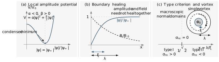
The material ledger of the minimal Ginzburg–Landau theory below $T_c$. The local potential selects a nonzero amplitude. Boundaries and defects force $|\psi|$ to heal over a scale set by $\xi$, while magnetic induction changes over $\lambda$. Their ratio $\kappa=\lambda/\xi$ controls the sign of the normal–superconducting interface energy and, in the single-component local bulk theory, separates type I from type II at $\kappa=1/\sqrt{2}$.

The Ginzburg–Landau parameter

The dimensionless ratio

$$\kappa \equiv \frac{\lambda}{\xi}$$

compares magnetic screening with amplitude healing. In the normalization used here,

$$\kappa^2 = \frac{ 2(m^\ast)^2\beta }{ \mu_0(q^\ast)^2\hbar^2 }.$$

The simple temperature dependences give

$$\lambda(T) \propto (T_c-T)^{-1/2},$$

and

$$\xi(T) \propto (T_c-T)^{-1/2},$$

so $\kappa$ approaches a constant near $T_c$ within mean-field GL theory.

At a flat boundary between normal and superconducting regions at the thermodynamic critical field, the interface energy changes sign at

$$\kappa_c = \frac{1}{\sqrt{2}}.$$

For the minimal local bulk model:

Regime	Interface energy	Flux organization
$\kappa<1/\sqrt{2}$	positive	type I; macroscopic normal and superconducting domains are favored
$\kappa=1/\sqrt{2}$	zero in the ideal model	Bogomolny point; special degeneracies occur
$\kappa>1/\sqrt{2}$	negative	type II; quantized vortices can form a mixed state

The criterion is exact for the ideal single-component isotropic GL model near its regime of validity. Multicomponent condensates, nonlocal electrodynamics, strong anisotropy, finite size, and interfaces can produce richer behavior. “Type-1.5” language, for example, requires more than inserting one effective $\lambda$ and one effective $\xi$ into the table.

Magnetic critical scales

Three field scales organize the ideal bulk problem. We report them in tesla using

$$B_{ci} \equiv \mu_0H_{ci}$$

for the ideal bulk geometry. In a shaped sample, internal induction, internal auxiliary field, and applied field must still be distinguished.

Thermodynamic critical field

The condensation-energy relation gave

$$B_c^2 = \mu_0 \frac{\alpha^2}{\beta}.$$

Using $\lambda$, $\xi$, and $\Phi_0$,

$$B_c = \frac{ \Phi_0 }{ 2\sqrt{2}\pi\lambda\xi }.$$

This identity follows from the chosen single-component GL normalization. It should not be used as an exact low-temperature identity in a material far outside the GL regime.

Upper critical field

Near the loss of superconductivity, $\psi$ is small, so the cubic term may be neglected:

$$\frac{1}{2m^\ast} \boldsymbol{\Pi}^2\psi + \alpha\psi =0.$$

In a uniform field, the kinetic operator has Landau levels. Its lowest transverse eigenvalue is

$$\frac{ \hbar|q^\ast|B }{ 2m^\ast }.$$

The normal state first becomes unstable when

$$\alpha + \frac{ \hbar|q^\ast|B_{c2} }{ 2m^\ast } =0.$$

Therefore

$$B_{c2} = \frac{ 2m^\ast|\alpha| }{ \hbar|q^\ast| } = \frac{ \Phi_0 }{ 2\pi\xi^2 }.$$

Combining results,

$$\frac{B_{c2}}{B_c} = \sqrt{2}\kappa.$$

The derivation is a direct material application of Landau Levels, but here the eigenfunction is the incipient order-parameter profile rather than a single-particle orbital.

Lower critical field

For a strongly type-II bulk superconductor,

$$\kappa\gg1,$$

the lower critical induction has the asymptotic form

$$B_{c1} \simeq \frac{ \Phi_0 }{ 4\pi\lambda^2 } \left( \ln\kappa+c_{\mathrm{core}} \right),$$

where the order-one constant $c_{\mathrm{core}}$ depends on the core treatment and approximation. Below $B_{c1}$, the equilibrium bulk state is Meissner-like. Between $B_{c1}$ and $B_{c2}$, flux enters as vortices in the ideal type-II picture.

These are equilibrium bulk scales. First penetration, irreversible magnetization, and resistive onset can occur at different fields because edge barriers, defects, pinning, vortex motion, sample shape, and the measurement criterion all matter.

Vortices as amplitude-resolving solutions

A vortex is possible because the phase winds while the amplitude vanishes at its core. Around a closed contour,

$$\oint \boldsymbol{\nabla}\theta\cdot \mathrm d\boldsymbol{\ell} = 2\pi N, \qquad N\in\mathbb Z.$$

For an isolated straight vortex along $\hat{\mathbf z}$, a cylindrically symmetric ansatz is

$$\psi(r,\varphi) = \psi_\infty f_N(r)e^{iN\varphi}.$$

Regularity requires

$$f_N(r) \propto r^{|N|}$$

near the origin, while

$$f_N(r)\longrightarrow1$$

far from the core. The core suppresses condensation energy over a scale of order $\xi$; circulating current and magnetic field extend over a scale of order $\lambda$.

Far from the core, where the current is negligible on a large contour, the gauge-invariant phase gradient gives

$$0 = 2\pi\hbar N - q^\ast\Phi.$$

Therefore the signed flux is

$$\Phi = \frac{h}{q^\ast}N = \operatorname{sgn}(q^\ast)N\Phi_0.$$

For an ordinary Cooper-pair field with $q^\ast=-2e$, this convention gives $\Phi=-N\Phi_0$; the flux magnitude is $|N|\Phi_0$, and reversing the winding reverses the flux orientation.

The London page states the more precise fluxoid relation. GL theory supplies the missing core where $\psi=0$, so a nonzero winding cannot be continuously unwound without crossing a configuration of vanishing amplitude or changing the boundary conditions.

For $\kappa\gg1$, the energy per unit length of a singly quantized vortex has the leading form

$$\varepsilon_v \simeq \frac{ \Phi_0^2 }{ 4\pi\mu_0\lambda^2 } \ln\kappa + \varepsilon_{\mathrm{core}}.$$

The logarithm comes from currents between the core and magnetic screening scales. The core contribution is not determined by a London calculation.

In the minimal type-II theory, well-separated singly quantized vortices repel and multiply quantized vortices generally split. Near $B_{c2}$, the linearized GL equation produces a highly degenerate lowest-Landau-level space. The quartic term selects a periodic Abrikosov lattice; in the ideal isotropic model, the triangular lattice minimizes

$$\beta_A \equiv \frac{ \langle|\psi|^4\rangle }{ \langle|\psi|^2\rangle^2 } \simeq 1.1596.$$

Real vortex matter is shaped by crystal anisotropy, nonlocality, disorder, pinning, thermal fluctuations, finite thickness, and drive. A vortex lattice seen in one probe does not imply a perfectly ordered equilibrium lattice throughout the sample.

Current-induced suppression

GL theory also captures amplitude suppression by superflow. Consider a region with uniform gauge-invariant condensate momentum

$$\mathbf p_s = \hbar\boldsymbol{\nabla}\theta - q^\ast\mathbf A.$$

The first GL equation gives

$$|\psi|^2 = \frac{ |\alpha|-p_s^2/(2m^\ast) }{ \beta }$$

while the current magnitude is

$$j_s = \frac{|q^\ast|}{m^\ast} |\psi|^2p_s.$$

Maximizing with respect to $p_s$ gives

$$p_s^2 = \frac{ 2m^\ast|\alpha| }{ 3 }.$$

The ideal GL depairing current density is

$$j_d = \frac{2\sqrt{2}}{3\sqrt{3}} \frac{ B_c }{ \mu_0\lambda }.$$

Because

$$B_c\propto(T_c-T), \qquad \lambda^{-1}\propto(T_c-T)^{1/2},$$

the mean-field scaling is

$$j_d \propto (T_c-T)^{3/2}.$$

Measured critical current is often much smaller. Vortex entry, phase slips, constrictions, weak links, heating, defects, and current crowding can trigger dissipation before the uniform depairing limit.

Near-transition scaling ledger

Under the elementary assumptions

$$\alpha=\alpha_0(T-T_c), \qquad \beta\approx\text{constant}, \qquad m^\ast\approx\text{constant},$$

mean-field GL theory predicts:

Quantity	Leading behavior below $T_c$
$\lvert\psi_\infty\rvert$	$(T_c-T)^{1/2}$
$\lvert\psi_\infty\rvert^2$	$T_c-T$
condensation energy density	$(T_c-T)^2$
$B_c$	$T_c-T$
$\xi$	$(T_c-T)^{-1/2}$
$\lambda$	$(T_c-T)^{-1/2}$
$B_{c2}$	$T_c-T$
$j_d$	$(T_c-T)^{3/2}$
$\kappa$	constant to leading order

These are mean-field asymptotics. A sufficiently narrow critical region is governed by fluctuations rather than the saddle point. In two dimensions, phase fluctuations and vortex unbinding can be especially important. A fit over a wide temperature interval should not be labeled a GL prediction merely because it uses the same powers.

Microscopic meaning and symmetry

Ginzburg and Landau introduced the theory phenomenologically. Gor’kov later derived its form from weak-coupling BCS theory near $T_c$ and showed that the covariant charge is twice the electronic charge. That derivation establishes an important logical relation:

$$\text{microscopic pairing theory} \quad\Longrightarrow\quad \text{GL coefficients in a controlled limit}.$$

It does not make the phenomenological coefficients universal. Band anisotropy, impurity scattering, multiple Fermi surfaces, strong coupling, and unconventional pairing change the coefficients and may require additional fields or invariants.

The order parameter transforms under a local gauge redundancy, but a redundancy is not an observable global symmetry that literally breaks. Physical statements should be phrased through gauge-invariant currents, fluxes, response functions, phase differences, and correlation functions. From Phase Symmetry to Gauge Theory owns that distinction.

Continue on QFT.org

This page stops at static material phenomenology. Landau–Ginzburg Theory Preview develops the regulated coarse-grained field, Gaussian fluctuations, correlation functions, interfaces, and Ginzburg criterion. Renormalization Group Preview explains scale dependence and the failure of mean-field exponents in a critical region.

Continue through the publication-aware QFT.org crosswalk and the live QFT.org hub when functional measures, gauge-field fluctuations, renormalized operators, universality classes, or relativistic Abelian Higgs theory become the main subject. Similar-looking functionals do not imply identical ensembles, dynamics, observables, or universality classes.

Extensions and limits

Anisotropic materials

Replace the scalar mass by a positive tensor:

$$f_{\mathrm{grad}} = \frac12 \left( \Pi_i\psi \right)^\ast \left( \mathsf M^{-1} \right)_{ij} \left( \Pi_j\psi \right).$$

Coherence lengths, penetration depths, $B_{c2}$, and vortex structures then depend on orientation. A single scalar $\kappa$ may be inadequate.

Multiple components and bands

Several complex fields can support:

• distinct amplitudes and healing lengths;
• interband Josephson-like couplings;
• relative-phase modes;
• domain walls and fractionalized defects under special conditions;
• competing or coexisting orders;
• nonmonotonic intervortex forces.

The allowed terms follow from crystal symmetry, time-reversal properties, gauge covariance, and the representation carried by the order parameter. One cannot obtain an unconventional GL theory by changing only the value of $m^\ast$.

Fluctuations and dimensionality

The equilibrium field configuration obtained by minimizing $F_{\mathrm{GL}}$ is a saddle-point or mean-field description. Thermal fluctuations require the statistical weight

$$Z = \int \mathcal D\psi\, \mathcal D\mathbf A\, \exp \left( - \frac{F_{\mathrm{GL}}}{ k_{\mathrm B}T } \right),$$

with a declared ultraviolet cutoff, gauge treatment, boundary conditions, and measure. Integrating over $\mathbf A$ is conceptually different from solving for a classical field profile.

Dynamics are not fixed by the static functional

The static GL functional does not uniquely determine time evolution. A time-dependent GL equation requires kinetic coefficients, conservation laws, noise, electromagnetic environment, and a regime of validity. Reactive condensate dynamics, relaxational critical dynamics, vortex flow, and microscopic nonequilibrium quasiparticles are different problems.

Low temperature and short scales

The elementary expansion can fail when:

• $T$ is far below $T_c$;
• variations occur on microscopic pair or lattice scales;
• nonlocal response matters;
• the gap has several components or nodes;
• strong pair breaking changes boundary physics;
• quantum fluctuations or nonequilibrium distributions dominate;
• the transition is first order or strongly inhomogeneous.

GL theory can remain a useful fitted effective model outside its strict asymptotic derivation, but then its accuracy must be established against observables rather than assumed.

Experimental inference workflow

1. Declare the ensemble and geometry. State applied-field orientation, sample dimensions, demagnetizing correction, and whether the observable is reversible.
2. Identify the transition. Establish that the relevant anomaly is superconducting and determine whether a continuous near-$T_c$ expansion is justified.
3. Measure independent scales. Infer $\lambda$, $\xi$, $B_c$, and $B_{c2}$ from observables with explicit model assumptions rather than solving every quantity from one fit.
4. Distinguish field criteria. Thermodynamic, magnetic-onset, torque, heat-capacity, and resistive definitions of a critical field need not coincide.
5. Check vortex contamination. Pinning and surface barriers can make first penetration differ from equilibrium $B_{c1}$.
6. Track orientation and anisotropy. Report tensor directions, not just one nominal GL parameter.
7. Restrict temperature extrapolation. A near-$T_c$ slope does not automatically determine a zero-temperature coherence length or critical field.
8. Test single-component locality. Multiband curvature, multiple gaps, nonlocal response, and competing order can invalidate the minimal model.
9. Propagate sample uncertainty. Surface damage, inclusions, thickness variation, current crowding, and heating can dominate inferred critical currents.
10. Use orthogonal probes. Combine thermodynamics, penetration depth, vortex imaging or scattering, spectroscopy, and transport.

Common mistakes

Mistake	Why it fails	Better practice
Calling $\psi$ a literal Cooper-pair wavefunction	It is a normalized coarse-grained order parameter	State its normalization and microscopic relation
Treating the phase as directly observable	$\theta$ is gauge dependent	Use covariant gradients, closed-loop winding, or phase differences
Dropping the magnetic field energy	$\mathbf A$ must be determined self-consistently	Vary both $\psi$ and $\mathbf A$ with boundary conditions
Using $\lvert\psi\rvert^2=-\alpha/\beta$ inside a vortex core	Gradient and magnetic terms are then essential	Solve the spatial GL equations
Calling every healing length $\xi$	Operational definitions can differ by factors such as $\sqrt{2}$	State the defining equation or profile
Classifying every material by one $\kappa$	Anisotropic or multicomponent systems can have several scales	Report the model and tensor or component structure
Equating first flux entry with $B_{c1}$	Barriers and demagnetization shift entry	Separate equilibrium and irreversible criteria
Using $B_{c2}=\Phi_0/(2\pi\xi^2)$ at all temperatures	It is a GL near-transition relation unless independently justified	State the fit window and extrapolation
Calling a resistive onset the thermodynamic transition	Vortex motion and inhomogeneity broaden transport	Compare magnetization and thermodynamics
Assuming static GL implies a unique TDGL equation	Dynamics require extra constitutive information	Specify kinetics, noise, and conservation laws
Extending mean-field exponents into the critical region	Fluctuations renormalize scaling	Estimate the Ginzburg region and test scaling
Treating gauge redundancy as broken global symmetry	Gauge-related fields describe the same physical state	Phrase claims in gauge-invariant observables

Exercises

1. Uniform minimum and condensation energy

For

$$f(u) = \alpha u + \frac{\beta}{2}u^2, \qquad u=|\psi|^2,$$

find the stable uniform state for $\alpha>0$ and $\alpha<0$, assuming $\beta>0$. Compute the condensation energy below $T_c$.

Solution

Differentiate with respect to the nonnegative variable $u$:

$$\frac{\mathrm df}{\mathrm du} = \alpha+\beta u.$$

For $\alpha>0$, the formal stationary point is negative and inaccessible, so the minimum is

$$u=0.$$

For $\alpha<0$,

$$u_\infty = - \frac{\alpha}{\beta}>0.$$

Substitution gives

$$\begin{aligned} f(u_\infty) &= \alpha \left( - \frac{\alpha}{\beta} \right) + \frac{\beta}{2} \left( \frac{\alpha^2}{\beta^2} \right) \\ &= - \frac{\alpha^2}{2\beta}. \end{aligned}$$

Taking the normal reference as zero, the condensation free-energy density is $-\alpha^2/(2\beta)$.

2. Derive the first GL equation

Vary the functional with respect to $\psi^\ast$ and recover the first GL equation. Assume boundary terms vanish.

Solution

The local terms vary as

$$\delta_{\psi^\ast} \left( \alpha|\psi|^2 + \frac{\beta}{2}|\psi|^4 \right) = \left( \alpha\psi + \beta|\psi|^2\psi \right) \delta\psi^\ast.$$

For the gradient term, covariant integration by parts gives

$$\delta_{\psi^\ast} \int \frac{ |\boldsymbol{\Pi}\psi|^2 }{ 2m^\ast } \mathrm d^3r = \int \delta\psi^\ast \frac{ \boldsymbol{\Pi}^2\psi }{ 2m^\ast } \mathrm d^3r.$$

Because $\delta\psi^\ast$ is arbitrary,

$$\frac{ \boldsymbol{\Pi}^2 }{ 2m^\ast } \psi + \alpha\psi + \beta|\psi|^2\psi =0.$$

3. Recover London screening

Set $\psi=\psi_\infty e^{i\theta}$ with constant amplitude. Derive the supercurrent and penetration depth.

Solution

Acting with the covariant momentum,

$$\boldsymbol{\Pi}\psi = e^{i\theta}\psi_\infty \left( \hbar\boldsymbol{\nabla}\theta - q^\ast\mathbf A \right).$$

The current is

$$\mathbf j_s = \frac{q^\ast}{m^\ast} |\psi_\infty|^2 \left( \hbar\boldsymbol{\nabla}\theta - q^\ast\mathbf A \right).$$

Away from singular phase winding,

$$\boldsymbol{\nabla}\times\mathbf j_s = - \frac{ (q^\ast)^2|\psi_\infty|^2 }{ m^\ast } \mathbf B.$$

Comparing with the second London equation gives

$$\lambda^2 = \frac{ m^\ast }{ \mu_0(q^\ast)^2|\psi_\infty|^2 }.$$

Using $|\psi_\infty|^2=|\alpha|/\beta$ gives the GL expression in the text.

4. Verify the planar healing profile

Show that

$$f(x) = \tanh \left( \frac{x}{ \sqrt{2}\xi } \right)$$

solves

$$- \xi^2f'' - f + f^3 =0.$$

Solution

Let

$$y = \frac{x}{ \sqrt{2}\xi }.$$

Then

$$f=\tanh y, \qquad \frac{\mathrm df}{\mathrm dy} = \operatorname{sech}^2y,$$

and

$$\frac{\mathrm d^2f}{\mathrm dy^2} = - 2\tanh y\, \operatorname{sech}^2y.$$

Because

$$\xi^2f'' = \frac12 \frac{\mathrm d^2f}{\mathrm dy^2} = - \tanh y\, \operatorname{sech}^2y,$$

the differential equation becomes

$$\tanh y\, \operatorname{sech}^2y - \tanh y + \tanh^3y.$$

Using

$$\operatorname{sech}^2y = 1-\tanh^2y,$$

the expression vanishes. The boundary values are $f(0)=0$ and $f(\infty)=1$.

5. Upper critical field from the lowest Landau level

Use the lowest eigenvalue of $\boldsymbol{\Pi}^2/(2m^\ast)$ in a uniform magnetic field to derive $B_{c2}$.

Solution

Near $B_{c2}$, the cubic term is negligible:

$$\left[ \frac{ \boldsymbol{\Pi}^2 }{ 2m^\ast } + \alpha \right] \psi =0.$$

The lowest transverse Landau energy is

$$E_0 = \frac{ \hbar|q^\ast|B }{ 2m^\ast }.$$

A nonzero solution first appears when

$$E_0+\alpha=0.$$

Since $\alpha<0$ below $T_c$,

$$B_{c2} = \frac{ 2m^\ast|\alpha| }{ \hbar|q^\ast| }.$$

With

$$\xi^2 = \frac{ \hbar^2 }{ 2m^\ast|\alpha| }, \qquad \Phi_0 = \frac{ 2\pi\hbar }{ |q^\ast| },$$

this becomes

$$B_{c2} = \frac{ \Phi_0 }{ 2\pi\xi^2 }.$$

6. Critical-field consistency

Show that

$$\frac{B_{c2}}{B_c} = \sqrt{2}\kappa.$$

What does this imply at $\kappa=1/\sqrt{2}$?

Solution

Use

$$B_{c2} = \frac{\Phi_0}{2\pi\xi^2}$$

and

$$B_c = \frac{ \Phi_0 }{ 2\sqrt{2}\pi\lambda\xi }.$$

Their ratio is

$$\frac{B_{c2}}{B_c} = \frac{ \Phi_0/(2\pi\xi^2) }{ \Phi_0/(2\sqrt{2}\pi\lambda\xi) } = \sqrt{2} \frac{\lambda}{\xi} = \sqrt{2}\kappa.$$

At $\kappa=1/\sqrt{2}$,

$$B_{c2}=B_c.$$

This coincides with the sign change of the normal–superconducting interface energy in the ideal model.

7. Flux of a singly quantized vortex

For a contour far from a vortex core, show that one unit of phase winding carries flux $h/|q^\ast|$ when the contour current is negligible.

Solution

Negligible current implies

$$\hbar\boldsymbol{\nabla}\theta - q^\ast\mathbf A \simeq0.$$

Integrate around the contour:

$$\hbar \oint \boldsymbol{\nabla}\theta\cdot \mathrm d\boldsymbol{\ell} - q^\ast \oint \mathbf A\cdot \mathrm d\boldsymbol{\ell} =0.$$

For winding $N=1$,

$$\oint \boldsymbol{\nabla}\theta\cdot \mathrm d\boldsymbol{\ell} = 2\pi,$$

and the second integral is the magnetic flux $\Phi$. Thus

$$q^\ast\Phi = 2\pi\hbar =h.$$

The orientation carries the sign, while the magnitude is

$$|\Phi| = \frac{h}{|q^\ast|} = \Phi_0.$$

8. Depairing-current scaling

Use the GL temperature scalings to determine the leading behavior of $j_d$ near $T_c$.

Solution

The ideal depairing current is

$$j_d = \frac{2\sqrt{2}}{3\sqrt{3}} \frac{ B_c }{ \mu_0\lambda }.$$

Near $T_c$,

$$B_c \propto T_c-T,$$

and

$$\lambda^{-1} \propto (T_c-T)^{1/2}.$$

Therefore

$$j_d \propto (T_c-T)^{3/2}.$$

This is the uniform mean-field depairing scale, not necessarily the transport critical current of a finite or disordered sample.

Connections

• Unconventional Superconductivity applies crystalline symmetry to multicomponent zero-momentum pairing representations and evidence for broken time reversal or nematicity; this page retains the spatial free-energy functional and its validity limits.
• London Theory owns local fixed-amplitude electrodynamics, penetration-depth geometry, fluxoid quantization, and nonlocality limits.
• Vortex Matter, Pinning, and Flux Flow takes the static core and Abrikosov solution developed here into collective elasticity, pinning, creep, melting or glass qualifications, and driven transport.
• Order Parameters owns source selection, thermodynamic limits, and the distinction between diagnostic fields and microscopic observables.
• Competing Orders extends local free-energy reasoning to coupled superconducting, magnetic, density-wave, and nematic orders, with coexistence and phase-topology tests.
• Pair-Density Waves and Exotic Orders extends superconducting order to finite momentum, composite charge-4e fields, and half-vortex–dislocation defects.
• Landau–Ginzburg Theory Preview owns the generic spatial functional, Gaussian response, interfaces, fluctuations, and Ginzburg criterion.
• BCS Theory owns the microscopic superconducting scales, observables, and weak-coupling limits that reduce to GL phenomenology near $T_c$.
• Superconducting Proximity Effect owns spatial anomalous propagation, inverse proximity, and Eilenberger–Usadel reductions outside the narrow near-$T_c$ local window in which this page’s boundary conditions apply.
• Moiré Superconductivity uses stiffness, vortex, critical-field, and BKT observables to test phase coherence in two-dimensional tunable condensates.
• Josephson Effect owns weak-link phase coupling, junction energy, interference, driven locking, and environmental phase dynamics.
• BCS Mean-Field Theory owns the microscopic paired saddle, gap equation, and quasiparticle spectrum from which GL coefficients can be derived near $T_c$.
• Off-Diagonal Long-Range Order distinguishes pair coherence from stiffness, spectral gaps, and electromagnetic response.
• Minimal Coupling in Wave Mechanics supplies the gauge-covariant momentum operator.
• Landau Levels supply the eigenvalue structure used in the $B_{c2}$ derivation.
• From Phase Symmetry to Gauge Theory explains global phase symmetry, local gauge covariance, and gauge redundancy.
• Susceptibilities owns response kernels, longitudinal and transverse limits, and internal-field corrections.

References

1. V. L. Ginzburg and L. D. Landau, “On the theory of superconductivity,” Zhurnal Eksperimental’noi i Teoreticheskoi Fiziki 20, 1064–1082 (1950); English translation in Collected Papers of L. D. Landau, 546–568 (1965), doi:10.1016/B978-0-08-010586-4.50078-X.
2. L. P. Gor’kov, “Microscopic derivation of the Ginzburg–Landau equations in the theory of superconductivity,” Soviet Physics JETP 9, 1364–1367 (1959), official JETP archive.
3. A. A. Abrikosov, “On the magnetic properties of superconductors of the second group,” Soviet Physics JETP 5, 1174–1182 (1957), official JETP archive.
4. A. A. Abrikosov, “Type-II superconductors and the vortex lattice,” Nobel Lecture (2003), NobelPrize.org.
5. P. G. de Gennes, Superconductivity of Metals and Alloys, Westview Press (1999).
6. M. Tinkham, Introduction to Superconductivity, 2nd ed., Dover (2004).
7. D. Saint-James, G. Sarma, and E. J. Thomas, Type II Superconductivity, Pergamon Press (1969).
8. E. H. Brandt, “The flux-line lattice in superconductors,” Reports on Progress in Physics 58, 1465–1594 (1995), doi:10.1088/0034-4885/58/11/003.
9. E. H. Brandt, “The vortex lattice in type-II superconductors: Ideal or distorted, in bulk and films,” physica status solidi (b) 248, 2305–2316 (2011), doi:10.1002/pssb.201147095.
10. J. R. Clem, “Simple model for the vortex core in a type II superconductor,” Journal of Low Temperature Physics 18, 427–434 (1975), doi:10.1007/BF00116134.
11. M. Sigrist and K. Ueda, “Phenomenological theory of unconventional superconductivity,” Reviews of Modern Physics 63, 239–311 (1991), doi:10.1103/RevModPhys.63.239.
12. R. L. Frank, C. Hainzl, R. Seiringer, and J. P. Solovej, “Microscopic derivation of Ginzburg–Landau theory,” Journal of the American Mathematical Society 25, 667–713 (2012), doi:10.1090/S0894-0347-2012-00735-8.
13. B. Rosenstein and D. Li, Ginzburg–Landau Theory of Condensates: Thermodynamics, Dynamics and Formation of Topological Matter, Cambridge University Press (2021), doi:10.1017/9781108872737.
14. A. Larkin and A. Varlamov, Theory of Fluctuations in Superconductors, Oxford University Press (2005), doi:10.1093/acprof:oso/9780198528159.001.0001.