BCS Theory

Bardeen–Cooper–Schrieffer theory explains how an arbitrarily weak attraction can destabilize a Fermi surface toward a coherent paired state and predicts the resulting excitation gap, thermodynamics, and electrodynamic rigidity. Its central achievement is not merely the existence of two-electron bound correlations. It is the self-consistent many-body state in which an extensive set of time-reversed orbitals participates coherently.

This page owns BCS as a theory of superconducting materials: what is assumed, which scales follow in the isotropic weak-coupling limit, how observables constrain those scales, and where the model must be generalized. BCS Mean-Field Theory owns the complete saddle-point derivation, Nambu matrix, gap and number equations, variational proof, and number-symmetry caveats. The Reduced BCS Model owns exact finite-level Richardson physics. Those pages are complements, not competing derivations.

Use the Superfluidity and Superconductivity gateway when the claim may instead require neutral-fluid, London, Ginzburg–Landau, vortex, Josephson, proximity, unconventional, or topological reasoning.

Required background. The many-body Fermi Surface supplies the low-energy shell and Pauli-blocked phase space, Density of States supplies the per-spin state-counting convention, Creation and Annihilation Operators supply the fermionic pairing algebra, and the Grand-Canonical Ensemble supplies chemical-potential bookkeeping.

Helpful background. The crystalline Fermi Surface supplies material pocket and multiband geometry, Phonons supplies one conventional retarded pairing route, and BCS Mean-Field Theory supplies the complete saddle derivation.

Scope and convention ledger

We begin with the clean, translationally invariant, single-band, spin-singlet, isotropic $s$-wave model. The reference normal state is a Fermi liquid with

$$\xi_{\mathbf k} = \varepsilon_{\mathbf k}-\mu.$$

Throughout:

• $e>0$ is the magnitude of the electron charge, so an electron carries charge $-e$;
• $N(0)$ is the normal-state density of states per spin at the Fermi energy and per unit volume;
• $V>0$ denotes the magnitude of an attractive matrix element, with the minus sign written explicitly in the Hamiltonian;
• $\hbar\omega_{\mathrm D}$ is a schematic pairing cutoff, not a claim that every phonon-mediated material has one sharp Debye mode;
• $\Delta$ is the isotropic mean-field pair potential;
• momentum sums include the normalization appropriate to the stated volume;
• the elementary weak-coupling formulas assume $N(0)V\ll1$ and $\hbar\omega_{\mathrm D}\ll E_{\mathrm F}$.

The per-spin convention matters. If $N_{\mathrm{tot}}(0)=2N(0)$ includes both spin projections, every formula containing a density of states must be converted consistently.

BCS has two useful meanings that should not be conflated:

1. BCS structure: a fermionic paired state described at mean-field level by an anomalous self-energy and Bogoliubov quasiparticles.
2. Elementary weak-coupling BCS limit: an isotropic, instantaneous reduced attraction with constant $N(0)$ and a sharp cutoff.

Many superconductors retain the first structure while violating the second model’s numerical ratios.

Why a Fermi surface is unstable

The normal Fermi sea has an exceptional phase-space geometry. Two fermions just above a filled Fermi sea can scatter between time-reversed states

$$(\mathbf k\uparrow,-\mathbf k\downarrow) \longrightarrow (\mathbf k'\uparrow,-\mathbf k'\downarrow)$$

without changing the pair’s total momentum. The large set of nearly degenerate pair states near the Fermi surface produces a logarithm in the pair susceptibility. Schematically,

$$\chi_{\mathrm{pair}}(T) \sim N(0) \int_{k_{\mathrm B}T}^{\hbar\omega_c} \frac{d\xi}{\xi} = N(0) \ln\left( \frac{\hbar\omega_c}{k_{\mathrm B}T} \right).$$

Consequently, the normal-state ladder sum develops a pole when

$$1-V\chi_{\mathrm{pair}}(T)=0.$$

No finite threshold in $V$ is required in the ideal Cooper channel. The resulting scale is exponentially small at weak coupling because it is generated by a logarithmic instability:

$$k_{\mathrm B}T_c \propto \hbar\omega_c \exp\left[ -\frac{1}{N(0)V} \right].$$

This statement is more specific than “attraction binds two particles.” The filled Fermi sea supplies Pauli blocking, a sharp low-energy manifold, and the logarithmic enhancement. BCS Mean-Field Theory owns the detailed Cooper instability and pair-wavefunction derivation. Unconventional Superconductivity extends this controlled isotropic baseline to zero-momentum crystal, pseudospin, and multiorbital pairing representations and their evidence audit. The essential many-body lesson here is that the instability reorganizes a shell of states around the entire Fermi surface.

Why phonons can mediate attraction

An electron deforms an ionic lattice; a second electron can couple to that delayed deformation. After the phonons are integrated out, the interaction is frequency dependent. In schematic Matsubara notation,

$$V_{\mathrm{eff}}(\mathbf q,i\Omega_n) = \lvert g_{\mathbf q}\rvert^2 D(\mathbf q,i\Omega_n),$$

where the phonon propagator $D$ is negative in the low-frequency convention relevant to the Cooper channel. The delayed attraction can evade part of the instantaneous screened Coulomb repulsion because electronic and ionic time scales differ.

The reduced BCS model replaces that retarded kernel by a constant attraction inside an energy shell. It is a controlled pedagogical reduction when retardation and spectral details are not themselves the observable. Phonons owns lattice quantization and phonon normal modes; strong-coupling retardation is treated below as an extension.

Reduced BCS Hamiltonian

Define a zero-center-of-mass pair operator

$$b_{\mathbf k}^\dagger = c_{\mathbf k\uparrow}^\dagger c_{-\mathbf k\downarrow}^\dagger.$$

The grand-canonical reduced Hamiltonian is

$$K \equiv H-\mu\hat N = \sum_{\mathbf k,\sigma} \xi_{\mathbf k} c_{\mathbf k\sigma}^\dagger c_{\mathbf k\sigma} - \sum_{\mathbf k,\mathbf k'} V_{\mathbf k\mathbf k'} b_{\mathbf k}^\dagger b_{\mathbf k'}.$$

For the elementary isotropic model,

$$V_{\mathbf k\mathbf k'} = \begin{cases} V, & \lvert\xi_{\mathbf k}\rvert, \lvert\xi_{\mathbf k'}\rvert < \hbar\omega_{\mathrm D}, \\ 0, & \text{otherwise}, \end{cases} \qquad V>0.$$

This reduction keeps scattering of time-reversed pairs and discards most other interaction channels. It does not prove that a microscopic material has an isotropic attraction, and it does not conserve the number of pairs in each orbital. The exact Hamiltonian does conserve total particle number:

$$[K,\hat N]=0.$$

The anomalous mean-field state introduced below does not have sharp particle number, but that is a representation of the thermodynamic paired phase, not a violation of microscopic charge conservation.

Pair field and mean-field state

Introduce the self-consistent pair potential

$$\Delta_{\mathbf k} = \sum_{\mathbf k'} V_{\mathbf k\mathbf k'} \left\langle c_{-\mathbf k'\downarrow} c_{\mathbf k'\uparrow} \right\rangle.$$

For isotropic $s$-wave pairing, $\Delta_{\mathbf k}=\Delta$ inside the active shell. The BCS variational state is

$$\lvert\mathrm{BCS}\rangle = \prod_{\mathbf k} \left( u_{\mathbf k} + v_{\mathbf k} c_{\mathbf k\uparrow}^\dagger c_{-\mathbf k\downarrow}^\dagger \right) \lvert0\rangle,$$

with

$$\lvert u_{\mathbf k}\rvert^2 + \lvert v_{\mathbf k}\rvert^2 =1.$$

Each momentum pair is a coherent superposition of empty and doubly occupied configurations. The product does not describe distinguishable, nonoverlapping molecular pairs. In the weak-coupling regime, many pair correlations overlap within a coherence volume.

A fixed-number state can be obtained by number projection:

$$\lvert\mathrm{BCS};N\rangle \propto \int_0^{2\pi} d\phi\, e^{-iN\phi/2} \prod_{\mathbf k} \left( u_{\mathbf k} + e^{i\phi} v_{\mathbf k} b_{\mathbf k}^\dagger \right) \lvert0\rangle.$$

Local bulk observables agree with the broken-symmetry description in the thermodynamic limit under the usual conditions. Finite isolated systems, parity effects, and exact level structure can require the number-conserving formulation.

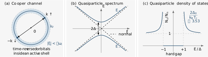
The elementary BCS ledger. (a) The reduced interaction couples time-reversed orbitals in a thin shell around the Fermi surface. (b) Pairing converts the normal crossing into Bogoliubov branches $E=\pm\sqrt{\xi^2+\Delta^2}$ separated by $2\Delta$. (c) An ideal isotropic gap removes states for $|E|<\Delta$ and produces integrable coherence-edge singularities. Broadening, anisotropy, nodes, and multiple bands reshape this last panel.

Bogoliubov quasiparticles

For one time-reversed block, the mean-field Hamiltonian has the Nambu matrix

$$\mathcal H_{\mathbf k} = \begin{pmatrix} \xi_{\mathbf k} & \Delta_{\mathbf k} \\ \Delta_{\mathbf k}^\ast & -\xi_{\mathbf k} \end{pmatrix}.$$

Its eigenvalues are

$$E_{\mathbf k,\pm} = \pm E_{\mathbf k}, \qquad E_{\mathbf k} = \sqrt{ \xi_{\mathbf k}^2 + \lvert\Delta_{\mathbf k}\rvert^2 }.$$

The positive branch is the physical quasiparticle excitation energy. The negative branch is the particle–hole partner in the doubled Nambu representation, not a second set of negative-energy particles.

For real positive $\Delta$, a convenient phase convention gives

$$\begin{aligned} \lvert u_{\mathbf k}\rvert^2 &= \frac12 \left( 1+\frac{\xi_{\mathbf k}}{E_{\mathbf k}} \right), \\ \lvert v_{\mathbf k}\rvert^2 &= \frac12 \left( 1-\frac{\xi_{\mathbf k}}{E_{\mathbf k}} \right), \\ u_{\mathbf k}v_{\mathbf k} &= \frac{\Delta}{2E_{\mathbf k}}. \end{aligned}$$

Far above the Fermi surface, a positive-energy quasiparticle is electron-like; far below, it is hole-like. Near $\xi_{\mathbf k}=0$, particle and hole amplitudes mix equally. Its charge expectation relative to the condensate is therefore momentum dependent:

$$q_{\mathbf k} = -e \left( \lvert u_{\mathbf k}\rvert^2 - \lvert v_{\mathbf k}\rvert^2 \right) = -e\frac{\xi_{\mathbf k}}{E_{\mathbf k}}.$$

Quasiparticle charge expectation is not a new conserved quantum number. Charge exchange with the condensate accompanies the particle–hole mixture. Bogoliubov Quasiparticles develops this operator structure across fermionic and bosonic systems.

Self-consistency and the gap equation

The anomalous thermal average is

$$\left\langle c_{-\mathbf k\downarrow} c_{\mathbf k\uparrow} \right\rangle = \frac{\Delta_{\mathbf k}}{2E_{\mathbf k}} \tanh\left( \frac{E_{\mathbf k}}{2k_{\mathrm B}T} \right).$$

Hence the general gap equation is

$$\Delta_{\mathbf k} = \sum_{\mathbf k'} V_{\mathbf k\mathbf k'} \frac{\Delta_{\mathbf k'}}{2E_{\mathbf k'}} \tanh\left( \frac{E_{\mathbf k'}}{2k_{\mathrm B}T} \right).$$

The isotropic constant-density-of-states reduction becomes

$$1 = N(0)V \int_0^{\hbar\omega_{\mathrm D}} \frac{d\xi}{ \sqrt{\xi^2+\Delta^2(T)} } \tanh\left[ \frac{ \sqrt{\xi^2+\Delta^2(T)} }{ 2k_{\mathrm B}T } \right].$$

The integral covers only $\xi>0$, which is why the per-spin $N(0)$ appears without an additional factor of two. This single convention prevents a common factor-of-two error.

The number equation must accompany the gap equation when density, rather than chemical potential, is fixed:

$$n = \frac{1}{\mathcal V} \sum_{\mathbf k} \left[ 1 - \frac{\xi_{\mathbf k}}{E_{\mathbf k}} \tanh\left( \frac{E_{\mathbf k}}{2k_{\mathrm B}T} \right) \right].$$

In a broad weak-coupling metal, $\mu$ shifts negligibly from $E_{\mathrm F}$. In a narrow band, dilute gas, or BCS–BEC crossover, solving only the gap equation can be qualitatively wrong.

Zero-temperature gap

At $T=0$,

$$\frac{1}{N(0)V} = \int_0^{\hbar\omega_{\mathrm D}} \frac{d\xi}{\sqrt{\xi^2+\Delta_0^2}} = \operatorname{arsinh} \left( \frac{\hbar\omega_{\mathrm D}}{\Delta_0} \right).$$

For $\Delta_0\ll\hbar\omega_{\mathrm D}$,

$$\Delta_0 \simeq 2\hbar\omega_{\mathrm D} \exp\left[ -\frac{1}{N(0)V} \right].$$

The exponential is nonanalytic at $V=0$: no finite-order perturbative expansion in $V$ can generate the gap.

Transition temperature

At $T_c$, linearize in $\Delta$:

$$\frac{1}{N(0)V} = \int_0^{\hbar\omega_{\mathrm D}} \frac{d\xi}{\xi} \tanh\left( \frac{\xi}{2k_{\mathrm B}T_c} \right).$$

In weak coupling,

$$k_{\mathrm B}T_c \simeq \frac{2e^{\gamma_{\mathrm E}}}{\pi} \hbar\omega_{\mathrm D} \exp\left[ -\frac{1}{N(0)V} \right],$$

where $\gamma_{\mathrm E}$ is Euler’s constant. Dividing the zero-temperature and transition scales removes the cutoff and coupling:

$$\frac{2\Delta_0}{k_{\mathrm B}T_c} = \frac{2\pi}{e^{\gamma_{\mathrm E}}} \simeq 3.528.$$

This number is a benchmark for the elementary isotropic weak-coupling model, not a universal definition of superconductivity.

Near $T_c$, the same model gives

$$\Delta(T) \simeq \sqrt{ \frac{8\pi^2}{7\zeta(3)} } k_{\mathrm B}T_c \sqrt{ 1-\frac{T}{T_c} } \simeq 3.06\,k_{\mathrm B}T_c \sqrt{ 1-\frac{T}{T_c} }.$$

The square-root onset is the microscopic source of the mean-field amplitude scaling used by Ginzburg–Landau Theory. Critical fluctuations can modify the asymptotic behavior sufficiently close to the transition.

Pair size and overlapping correlations

A useful weak-coupling length is the Pippard–BCS coherence length

$$\xi_0 = \frac{\hbar v_{\mathrm F}}{\pi\Delta_0}.$$

It estimates the spatial range of pair correlations and the nonlocal electrodynamic kernel in a clean isotropic metal. For an isotropic parabolic band,

$$k_{\mathrm F}\xi_0 = \frac{2E_{\mathrm F}}{\pi\Delta_0},$$

ordinary weak-coupling metals have $k_{\mathrm F}\xi_0\gg1$. The pair size is therefore much larger than the interparticle spacing, and a coherence volume contains many strongly overlapping pair correlations.

Several lengths called “coherence length” coexist:

Symbol or method	Meaning	Typical regime
$\xi_0=\hbar v_{\mathrm F}/(\pi\Delta_0)$	Clean weak-coupling Pippard–BCS pair-correlation scale	Low-temperature microscopic theory
$\xi_{\mathrm{GL}}(T)$	Order-parameter healing length	Near a continuous $T_c$
$\sqrt{\Phi_0/(2\pi B_{c2})}$	Field-inferred effective length	GL regime or an explicitly justified extrapolation
$\sqrt{\hbar D/\Delta}$	Diffusive coherence scale, up to convention-dependent factors	Dirty limit

These quantities can be related in controlled limits, but they are not interchangeable definitions.

Thermodynamic signatures

Condensation energy

At $T=0$, the weak-coupling free-energy density difference is

$$f_s-f_n = -\frac12 N(0)\Delta_0^2.$$

With the present per-spin convention, the normal-state Sommerfeld coefficient is

$$\gamma_n = \frac{2\pi^2}{3} k_{\mathrm B}^2N(0), \qquad C_n=\gamma_n T.$$

Thus

$$\frac{f_n-f_s}{\gamma_nT_c^2} = \frac{3}{4\pi^2} \left( \frac{\Delta_0}{k_{\mathrm B}T_c} \right)^2 \simeq 0.236.$$

For an ideal bulk sample in SI units, the same energy defines the thermodynamic critical induction:

$$\frac{B_c^2(0)}{2\mu_0} = \frac12N(0)\Delta_0^2.$$

This is a thermodynamic relation. The first resistive field, first flux-entry field, and upper critical field are different observables.

Specific-heat jump

The quasiparticle entropy can be written

$$S_s = -2k_{\mathrm B} \sum_{\mathbf k} \left[ f_{\mathbf k}\ln f_{\mathbf k} + (1-f_{\mathbf k}) \ln(1-f_{\mathbf k}) \right],$$

where $f_{\mathbf k}=f(E_{\mathbf k})$. Differentiation, including the temperature dependence of $\Delta(T)$, gives the weak-coupling jump

$$\frac{ C_s(T_c^-)-C_n(T_c^+) }{ \gamma_nT_c } = \frac{12}{7\zeta(3)} \simeq 1.426.$$

At $T\ll T_c$, a clean fully gapped state has exponentially suppressed electronic heat capacity. Nodes instead produce power laws whose exponents depend on dimensionality, nodal geometry, disorder, and the measured response.

The number $1.426$ is a model benchmark. A different jump can arise from strong coupling, gap anisotropy, multiple bands, partial superconducting volume, transition broadening, or an incorrectly subtracted phonon background.

Spectroscopic and response signatures

Quasiparticle density of states

For a clean isotropic gap,

$$\frac{N_s(E)}{N_n(0)} = \operatorname{Re} \frac{\lvert E\rvert}{ \sqrt{E^2-\Delta^2} }.$$

The ideal model has:

• no single-particle states for $\lvert E\rvert<\Delta$;
• integrable square-root singularities at $\lvert E\rvert=\Delta$;
• recovery of the normal density of states for $\lvert E\rvert\gg\Delta$.

A commonly used phenomenological broadening is the Dynes form

$$\frac{N_\Gamma(E)}{N_n(0)} = \operatorname{Re} \frac{E+i\Gamma}{ \sqrt{(E+i\Gamma)^2-\Delta^2} }.$$

$\Gamma$ is a fit parameter, not automatically a microscopic scattering rate. Energy resolution, temperature, spatial inhomogeneity, anisotropy, several gaps, pair breaking, and genuine lifetime effects can produce similar rounding.

Tunneling is a convolution

For a normal-metal tip with slowly varying density of states,

$$\frac{dI}{dV}(V) \propto \int_{-\infty}^{\infty} dE\, N_s(E) \left[ -\frac{\partial f(E-eV)}{\partial E} \right].$$

Only in the low-temperature, energy-independent-tip limit does $dI/dV$ closely trace $N_s(eV)$. A superconducting tip introduces a second gapped density of states and shifts the dominant thresholds. Matrix elements and nonequilibrium effects can matter as well.

Scanning Tunneling Microscopy and Spectroscopy owns the junction calibration, resolution convolution, setpoint effects, spatial gap fitting, and defect and vortex maps needed to apply this spectrum experimentally.

Coherence factors matter

BCS response is not determined by the density of states alone. A probe can couple to combinations such as

$$u_{\mathbf k}u_{\mathbf k'} \mp v_{\mathbf k}v_{\mathbf k'},$$

and the sign depends on the vertex, momentum transfer, and relative gap phase. These coherence factors explain why charge, spin, ultrasound, electromagnetic, and nuclear-relaxation probes need not show the same threshold structure.

Canonical weak-coupling signatures include:

Probe	Elementary isotropic expectation	Important caveat
Tunneling	Gap edges near $\pm\Delta/e$ with coherence peaks	Thermal convolution, matrix elements, broadening, anisotropy
Heat capacity	Jump $1.426\,\gamma_nT_c$ and activated low-$T$ tail	Phonon subtraction, multiband structure, volume fraction
NMR relaxation	Possible Hebel–Slichter peak, then activated suppression	Disorder, fields, inelastic scattering, and correlations can remove the peak
Penetration depth	Exponentially small low-$T$ correction for a full gap	Surface state, nonlocality, disorder, and gap minima
Optical response	Missing low-frequency spectral weight and a condensate delta function	Pair-breaking threshold and line shape depend on scattering and vertex physics
Isotope substitution	$\alpha\simeq1/2$ in the simplest phonon model	Coulomb retardation, anharmonicity, several modes, and structural changes

No single row proves the pairing mechanism. Trustworthy identification combines thermodynamics, spectroscopy, magnetic response, isotope or pressure trends, and sample characterization.

Electrodynamic rigidity and phase

The pair field has an amplitude and phase,

$$\Delta(\mathbf r) = \lvert\Delta(\mathbf r)\rvert e^{i\theta(\mathbf r)}.$$

A spatially coherent phase gives a nonzero transverse electromagnetic stiffness. Microscopic BCS theory yields a current-response kernel that reduces to London electrodynamics in the long-wavelength, low-frequency limit:

$$\mathbf j_s \simeq -\frac{1}{\mu_0\lambda^2} \left( \mathbf A + \frac{\hbar}{2e} \boldsymbol{\nabla}\theta \right),$$

where $\Delta\propto\langle cc\rangle$ and $\mathbf A\to\mathbf A+\boldsymbol{\nabla}\chi$ imply $\theta\to\theta-2e\chi/\hbar$. The combination in parentheses is therefore gauge invariant.

The electromagnetic gauge redundancy is not itself an observable global symmetry that literally breaks. Measurable statements concern stiffness, flux quantization, current, phase differences, correlation functions, and the electromagnetic spectrum. London Theory owns penetration and fluxoid geometry; Off-Diagonal Long-Range Order owns number-conserving coherence diagnostics.

Pair formation and superconducting phase coherence can also occur at different scales. Elementary weak-coupling metals have a large phase stiffness, so amplitude formation controls $T_c$. Low-density, quasi-two-dimensional, granular, or strongly fluctuating systems can instead be limited by phase ordering.

From the isotope effect to Eliashberg theory

In the elementary model,

$$T_c \propto \omega_{\mathrm D} \exp\left[ -\frac{1}{N(0)V} \right].$$

If only the ionic mass $M$ changes and $\omega_{\mathrm D}\propto M^{-1/2}$ while $N(0)V$ remains fixed, the isotope exponent is

$$\alpha_{\mathrm{iso}} \equiv -\frac{d\ln T_c}{d\ln M} = \frac12.$$

The mercury isotope effect was decisive historical evidence for lattice participation, but $\alpha_{\mathrm{iso}}\ne1/2$ does not by itself rule phonons out. The pairing interaction, phonon spectrum, Coulomb pseudopotential, anharmonicity, and even crystal structure may change under isotope substitution.

Retardation reduces the effective low-energy Coulomb repulsion. A schematic Morel–Anderson form is

$$\mu^\ast = \frac{\mu}{ 1+\mu \ln\left( \dfrac{E_{\mathrm{el}}}{ \hbar\omega_{\mathrm{ph}} } \right) }.$$

Migdal–Eliashberg theory retains the frequency-dependent electron and gap self-energies. Its material input is the electron–phonon spectral function $\alpha^2F(\omega)$, from which one defines

$$\lambda_{\mathrm{ep}} = 2 \int_0^\infty d\omega\, \frac{\alpha^2F(\omega)}{\omega},$$

and

$$\ln\omega_{\log} = \frac{2}{\lambda_{\mathrm{ep}}} \int_0^\infty d\omega\, \frac{\alpha^2F(\omega)}{\omega} \ln\omega.$$

The Allen–Dynes refinement of McMillan’s interpolation is commonly written

$$k_{\mathrm B}T_c \simeq \frac{ f_1f_2\hbar\omega_{\log} }{1.20} \exp\left[ - \frac{ 1.04(1+\lambda_{\mathrm{ep}}) }{ \lambda_{\mathrm{ep}} - \mu^\ast (1+0.62\lambda_{\mathrm{ep}}) } \right].$$

This is an interpolation within a phonon-mediated Eliashberg setting, not a universal transition-temperature law. Its use requires a defensible $\alpha^2F$, Coulomb parameter, phonon stability, and regime where neglected vertex corrections remain controlled.

Worked material-scale inference

Suppose a bulk sample has

$$T_c=10.0\ \mathrm K, \qquad \Delta_0=1.90\ \mathrm{meV}, \qquad v_{\mathrm F}=3.0\times10^5\ \mathrm{m\,s^{-1}}.$$

Using $k_{\mathrm B}=0.08617\ \mathrm{meV\,K^{-1}}$,

$$\frac{2\Delta_0}{k_{\mathrm B}T_c} = \frac{3.80}{0.8617} \simeq 4.41.$$

That ratio lies above the elementary weak-coupling value $3.528$. It motivates tests for strong coupling, anisotropy, multiple gaps, and experimental broadening; it does not identify which explanation is correct.

The clean Pippard–BCS estimate is

$$\begin{aligned} \xi_0 &= \frac{\hbar v_{\mathrm F}}{\pi\Delta_0} \\ &\simeq \frac{ (6.582\times10^{-16}\ \mathrm{eV\,s}) (3.0\times10^5\ \mathrm{m\,s^{-1}}) }{ \pi(1.90\times10^{-3}\ \mathrm{eV}) } \\ &\simeq 33\ \mathrm{nm}. \end{aligned}$$

This estimate should not be reported as the GL healing length without an independent regime-specific relation. A measured $B_{c2}$, penetration depth, residual resistivity, and band-resolved velocity would determine whether clean single-band BCS is even an adequate comparison.

Experimental inference workflow

1. Establish bulk superconductivity. Combine zero resistance with magnetic screening or a thermodynamic anomaly; transport alone can be short-circuited by a minority path.
2. Declare the normal reference. State how the electronic heat capacity, normal density of states, and background conductivity were obtained.
3. Measure more than one gap-sensitive observable. Compare tunneling, heat capacity, penetration depth, terahertz or infrared conductivity, thermal transport, or NMR.
4. Fit the forward model. Convolve the density of states with temperature, instrumental resolution, tip spectrum, and matrix elements before assigning $\Delta$.
5. Test gap structure. Look for consistent exponential or power-law behavior over a controlled low-temperature window and across disorder or field.
6. Check thermodynamic closure. Compare entropy balance, condensation energy, $\gamma_n$, and critical-field data.
7. Separate pair and phase scales. In low-stiffness systems, determine whether fluctuations or vortex physics broaden the transition.
8. Resolve band and momentum dependence. A single fitted gap can hide several bands or strong anisotropy.
9. Audit disorder and volume fraction. Pair breaking, inhomogeneity, surfaces, and nonsuperconducting fractions can mimic unconventional behavior.
10. Use isotope or pressure data carefully. Verify that substitution or pressure has not changed structure, carrier density, or competing order.
11. Compare model ratios last. Ratios such as $2\Delta_0/(k_{\mathrm B}T_c)$ are diagnostics after the measurement model is trusted, not stand-alone labels.

Limitations and generalizations

Retardation and strong coupling

The elementary reduced interaction is instantaneous. Real phonon-mediated pairing has frequency-dependent self-energies, mass renormalization, damping, and a structured spectrum. Eliashberg theory can predict deviations from weak-coupling ratios and spectroscopic structures tied to phonon energies.

Anisotropic and sign-changing gaps

Crystal symmetry permits momentum-dependent basis functions:

$$\Delta(\mathbf k) = \sum_a \eta_a\phi_a(\mathbf k).$$

Nodes, deep minima, and sign changes alter low-energy thermodynamics and coherence factors. A nodeless density of states does not establish isotropic $s$-wave pairing, and a sign-changing state may still have a full gap on every Fermi-surface sheet.

Multiband superconductivity

Several Fermi surfaces require a matrix gap equation,

$$\Delta_i = \sum_j \lambda_{ij} \Delta_j \mathcal L_j(T,\Delta_j).$$

Here $\mathcal L_j$ is the dimensionless pair kernel on band $j$. Interband coupling can lock relative phases while preserving distinct gap magnitudes. Thermodynamic and spectroscopic probes weight bands differently, so one “measured gap” need not represent the whole material.

Disorder and pair breaking

Nonmagnetic disorder leaves $T_c$ comparatively robust in an ideal isotropic $s$-wave state under Anderson’s theorem assumptions, but it changes transport and the clean/dirty electrodynamic regime. Magnetic impurities, sign-changing gaps, strong inhomogeneity, localization, or correlated disorder can suppress pairing and create subgap states.

Low density and the BCS–BEC crossover

When $\Delta/E_{\mathrm F}$ is no longer small, $\mu$ must be solved self-consistently and can move substantially. Pair size approaches the interparticle spacing, pair formation can precede condensation, and the weak-coupling Fermi-surface logarithm is no longer the whole story.

Phase fluctuations and dimensionality

Mean field determines the amplitude saddle. It can overestimate the actual transition when superfluid stiffness is small. In two dimensions, vortex unbinding can govern phase coherence even when a local pairing amplitude exists above the transition.

Non-Fermi-liquid normal states

The elementary derivation assumes coherent normal-state quasiparticles and a controlled attractive vertex. Strong correlations, competing order, pseudogaps, and incoherent spectral weight can invalidate that starting point. A successful BCS-shaped fit to the superconducting spectrum does not by itself establish a weakly interacting normal state or a phonon mechanism.

Common mistakes

Mistake	Why it fails	Better practice
Calling every pair a small molecule	Weak-coupling pairs overlap over $\xi_0\gg k_{\mathrm F}^{-1}$	Report $k_{\mathrm F}\xi_0$ or $\Delta/E_{\mathrm F}$
Saying the reduced Hamiltonian violates number conservation	The exact quartic Hamiltonian commutes with $\hat N$	Distinguish it from the anomalous mean-field saddle
Counting both Nambu branches as independent particles	Nambu space doubles the representation	Keep one positive-energy quasiparticle branch per physical mode
Mixing per-spin and total density of states	It changes gap and condensation-energy prefactors	State the convention before integrating
Treating $\Delta$ as every experimental gap	Spectral edges, order parameters, pseudogaps, and band gaps can differ	Define the observable and forward model
Calling $3.528$ universal	It assumes isotropic weak coupling and a simple cutoff	Use it as a benchmark, then test corrections
Reading tunneling conductance directly as $N_s(eV)$	Finite temperature and the tip spectrum cause convolution	Fit the full tunneling expression
Inferring nodes from one power law	Disorder, surfaces, vortices, and crossover windows can imitate powers	Compare several bulk probes over controlled ranges
Taking the absence of a Hebel–Slichter peak as proof of unconventional pairing	Fields, disorder, inelastic scattering, and correlations suppress it	Model the relaxation vertex and sample conditions
Identifying $\alpha_{\mathrm{iso}}\ne1/2$ with nonphononic pairing	$\mu^\ast$, anharmonicity, several modes, and structural shifts modify $\alpha$	Track the full phonon and electronic changes
Equating pair formation with zero resistance	Global phase coherence and vortex dynamics are additional requirements	Measure stiffness, screening, and thermodynamics
Treating gauge redundancy as an observable broken symmetry	Gauge-related fields describe the same physical state	Use currents, fluxes, phase differences, and correlators
Using McMillan–Allen–Dynes outside its domain	It is a phonon-Eliashberg interpolation	Verify phonons, stability, coupling regime, and spectral input

Exercises

1. Derive the zero-temperature weak-coupling gap

Starting from

$$\frac{1}{N(0)V} = \int_0^{\hbar\omega_{\mathrm D}} \frac{d\xi}{ \sqrt{\xi^2+\Delta_0^2} },$$

evaluate the integral exactly and obtain the weak-coupling asymptote.

Solution

Use

$$\int \frac{d\xi}{\sqrt{\xi^2+\Delta_0^2}} = \operatorname{arsinh} \left( \frac{\xi}{\Delta_0} \right).$$

Therefore

$$\frac{1}{N(0)V} = \operatorname{arsinh} \left( \frac{\hbar\omega_{\mathrm D}}{\Delta_0} \right).$$

Inverting exactly gives

$$\Delta_0 = \frac{ \hbar\omega_{\mathrm D} }{ \sinh[1/(N(0)V)] }.$$

For $N(0)V\ll1$,

$$\sinh\left[ \frac{1}{N(0)V} \right] \simeq \frac12 \exp\left[ \frac{1}{N(0)V} \right],$$

so

$$\Delta_0 \simeq 2\hbar\omega_{\mathrm D} e^{-1/[N(0)V]}.$$

The essential singularity at $V=0$ records the nonperturbative Cooper instability.

2. Eliminate the microscopic cutoff

Use the weak-coupling expressions for $\Delta_0$ and $T_c$ to derive $2\Delta_0/(k_{\mathrm B}T_c)$.

Solution

The two scales are

$$\Delta_0 = 2\hbar\omega_{\mathrm D} e^{-1/[N(0)V]},$$

and

$$k_{\mathrm B}T_c = \frac{2e^{\gamma_{\mathrm E}}}{\pi} \hbar\omega_{\mathrm D} e^{-1/[N(0)V]}.$$

Their ratio is therefore

$$\frac{2\Delta_0}{k_{\mathrm B}T_c} = \frac{ 4\hbar\omega_{\mathrm D} e^{-1/[N(0)V]} }{ (2e^{\gamma_{\mathrm E}}/\pi) \hbar\omega_{\mathrm D} e^{-1/[N(0)V]} } = \frac{2\pi}{e^{\gamma_{\mathrm E}}} \simeq 3.528.$$

The cancellation works only because both formulas use the same interaction, cutoff, and weak-coupling approximation.

3. Close the condensation-energy ledger

Given the per-spin convention

$$\gamma_n = \frac{2\pi^2}{3}k_{\mathrm B}^2N(0),$$

show that weak-coupling BCS predicts

$$\frac{f_n-f_s}{\gamma_nT_c^2} \simeq 0.236.$$

Solution

From $f_n-f_s=N(0)\Delta_0^2/2$,

$$\frac{f_n-f_s}{\gamma_nT_c^2} = \frac{ N(0)\Delta_0^2/2 }{ (2\pi^2/3) k_{\mathrm B}^2N(0)T_c^2 } = \frac{3}{4\pi^2} \left( \frac{\Delta_0}{k_{\mathrm B}T_c} \right)^2.$$

Using $\Delta_0/(k_{\mathrm B}T_c)=\pi/e^{\gamma_{\mathrm E}}\simeq1.764$ gives

$$\frac{f_n-f_s}{\gamma_nT_c^2} \simeq \frac{3(1.764)^2}{4\pi^2} \simeq 0.236.$$

Had $N(0)$ been interpreted as the two-spin density of states, the starting condensation-energy prefactor would have needed conversion.

4. Quasiparticle charge near the Fermi surface

Derive the charge expectation

$$q_{\mathbf k} = -e\frac{\xi_{\mathbf k}}{E_{\mathbf k}}$$

and interpret its three limits $\xi_{\mathbf k}\gg\Delta$, $\xi_{\mathbf k}=0$, and $\xi_{\mathbf k}\ll-\Delta$.

Solution

A normalized quasiparticle mixes an electron component of weight $\lvert u_{\mathbf k}\rvert^2$ and a hole component of weight $\lvert v_{\mathbf k}\rvert^2$. Relative to the condensate,

$$q_{\mathbf k} = (-e)\lvert u_{\mathbf k}\rvert^2 + (+e)\lvert v_{\mathbf k}\rvert^2 = -e \left( \lvert u_{\mathbf k}\rvert^2 - \lvert v_{\mathbf k}\rvert^2 \right).$$

Since

$$\lvert u_{\mathbf k}\rvert^2 - \lvert v_{\mathbf k}\rvert^2 = \frac{\xi_{\mathbf k}}{E_{\mathbf k}},$$

the result follows. Far above the Fermi surface $q_{\mathbf k}\to-e$; at the Fermi surface the expectation vanishes because electron and hole weights are equal; far below it tends to $+e$. This is an expectation value, not a sharp quasiparticle charge eigenvalue.

5. Resolve an ideal coherence edge

Let $E=\Delta+\epsilon$ with $0<\epsilon\ll\Delta$. Find the leading divergence of the ideal BCS density of states. Then evaluate the normalized Dynes density of states at $E=0$.

Solution

Near the positive edge,

$$E^2-\Delta^2 = (\Delta+\epsilon)^2-\Delta^2 \simeq 2\Delta\epsilon.$$

Thus

$$\frac{N_s(E)}{N_n(0)} \simeq \frac{\Delta}{ \sqrt{2\Delta\epsilon} } = \sqrt{ \frac{\Delta}{2\epsilon} }.$$

The divergence is integrable because its integral scales as $\sqrt{\epsilon}$.

For the Dynes form,

$$\frac{N_\Gamma(0)}{N_n(0)} = \operatorname{Re} \frac{i\Gamma}{ \sqrt{-\Gamma^2-\Delta^2} } = \frac{\Gamma}{ \sqrt{\Gamma^2+\Delta^2} },$$

with the retarded square-root branch. Broadening fills the ideal hard gap, but this phenomenological result does not uniquely identify the broadening mechanism.

6. Interpret a heat-capacity jump

A sample has $T_c=8.0\ \mathrm K$ and $\gamma_n=25\ \mathrm{mJ\,mol^{-1}K^{-2}}$. Compute the elementary BCS jump. Explain why agreement with that number would not prove phonon-mediated isotropic pairing.

Solution

The weak-coupling prediction is

$$\Delta C = 1.426\,\gamma_nT_c.$$

Therefore

$$\Delta C \simeq 1.426 (25\ \mathrm{mJ\,mol^{-1}K^{-2}}) (8.0\ \mathrm K) \simeq 285\ \mathrm{mJ\,mol^{-1}K^{-1}}.$$

The jump is an integrated thermodynamic constraint, not a direct measurement of gap phase or pairing glue. Anisotropy, several bands, coupling corrections, nonsuperconducting volume, and background subtraction can compensate one another and produce an apparently BCS-like ratio.

7. Generalize the isotope exponent

Assume

$$T_c = C M^{-1/2} \exp[-1/\lambda(M)]$$

and define $\beta=d\ln\lambda/d\ln M$. Derive the isotope exponent $\alpha_{\mathrm{iso}}$.

Solution

Take a logarithm:

$$\ln T_c = \ln C - \frac12\ln M - \frac{1}{\lambda}.$$

Differentiating gives

$$\frac{d\ln T_c}{d\ln M} = -\frac12 + \frac{1}{\lambda^2} \frac{d\lambda}{d\ln M} = -\frac12 + \frac{\beta}{\lambda}.$$

Hence

$$\alpha_{\mathrm{iso}} \equiv -\frac{d\ln T_c}{d\ln M} = \frac12 - \frac{\beta}{\lambda}.$$

The textbook value $1/2$ requires mass-independent dimensionless coupling. Coulomb retardation, spectral redistribution, anharmonicity, and structural isotope effects add further corrections.

8. Are weak-coupling pairs molecular?

Show that

$$k_{\mathrm F}\xi_0 = \frac{2E_{\mathrm F}}{\pi\Delta_0}.$$

Estimate it for $\Delta_0/E_{\mathrm F}=10^{-3}$ and interpret the result.

Solution

For a parabolic band,

$$v_{\mathrm F} = \frac{\hbar k_{\mathrm F}}{m}, \qquad E_{\mathrm F} = \frac{\hbar^2k_{\mathrm F}^2}{2m}.$$

Multiplying $\xi_0=\hbar v_{\mathrm F}/(\pi\Delta_0)$ by $k_{\mathrm F}$ gives

$$k_{\mathrm F}\xi_0 = \frac{\hbar^2k_{\mathrm F}^2}{ \pi m\Delta_0 } = \frac{2E_{\mathrm F}}{\pi\Delta_0}.$$

For $\Delta_0/E_{\mathrm F}=10^{-3}$,

$$k_{\mathrm F}\xi_0 = \frac{2}{\pi\times10^{-3}} \simeq 637.$$

The pair-correlation length is hundreds of inverse Fermi wavevectors. Many pairs overlap in real space, so the weak-coupling state is not a dilute gas of compact, distinguishable molecules.

Connections

• BCS Mean-Field Theory owns the full anomalous decoupling, Nambu diagonalization, variational state, gap and number equations, grand potential, and symmetry logic.
• Reduced BCS Model owns exact number-conserving finite-level pairing, Richardson roots, blocking, and parity effects.
• Bogoliubov Quasiparticles compares fermionic and bosonic canonical transformations and the meaning of particle–hole mixing.
• Density of States owns state counting, dimensional singularities, and per-volume conventions in crystalline bands.
• Phonons owns the quantized lattice excitations that can mediate retarded attraction.
• Heat Capacity and Thermodynamics owns calorimetric extraction of $\gamma_n$, entropy balance, transition anomalies, addenda, and background systematics.
• Moiré Superconductivity applies the conventional benchmark to narrow multicomponent bands, BKT-limited coherence, quantum-geometric stiffness, and competing pairing mechanisms.
• Disorder in Quantum Matter defines the quenched potentials, elastic lifetimes, and clean-to-dirty transport scales presupposed by disorder tests of pairing.
• Off-Diagonal Long-Range Order gives a number-conserving criterion for pair coherence and distinguishes it from a spectral gap or stiffness.
• Ginzburg–Landau Theory owns spatial order-parameter phenomenology, critical fields, type classification, and vortex cores near $T_c$.
• Pair-Density Waves and Exotic Orders generalizes the uniform pairing benchmark to finite center-of-mass momentum, composite orders, and phase-sensitive evidence.
• London Theory owns local fixed-amplitude electrodynamics, penetration geometry, and fluxoid quantization.
• Superconducting Proximity Effect takes the homogeneous parent gap into spatial anomalous propagation, inverse proximity, and controlled clean or diffusive reductions; this page retains the uniform material BCS benchmark.
• Proximity and Andreev Physics carries the BCS gap into normal–superconductor scattering, induced pairing, transmission-resolved bound states, and hybrid-device diagnostics.
• Josephson Effect owns coherent weak-link transport, phase-sensitive current, voltage–frequency locking, SQUIDs, and junction circuit dynamics.
• Topological Superconductors begins where the conventional pairing framework ends: BdG invariants, Majorana boundary and vortex modes, and the evidence required of candidate platforms.
• Spectral Functions supplies the language needed when self-energy, lifetime, and incoherent weight replace an ideal BCS density of states.

References

1. J. Bardeen, L. N. Cooper, and J. R. Schrieffer, “Theory of Superconductivity,” Physical Review 108, 1175–1204 (1957), doi:10.1103/PhysRev.108.1175.
2. L. N. Cooper, “Bound Electron Pairs in a Degenerate Fermi Gas,” Physical Review 104, 1189–1190 (1956), doi:10.1103/PhysRev.104.1189.
3. H. Fröhlich, “Theory of the Superconducting State. I. The Ground State at the Absolute Zero of Temperature,” Physical Review 79, 845–856 (1950), doi:10.1103/PhysRev.79.845.
4. E. Maxwell, “Isotope Effect in the Superconductivity of Mercury,” Physical Review 78, 477 (1950), doi:10.1103/PhysRev.78.477.
5. C. A. Reynolds, B. Serin, W. H. Wright, and L. B. Nesbitt, “Superconductivity of Isotopes of Mercury,” Physical Review 78, 487 (1950), doi:10.1103/PhysRev.78.487.
6. I. Giaever, “Energy Gap in Superconductors Measured by Electron Tunneling,” Physical Review Letters 5, 147–148 (1960), doi:10.1103/PhysRevLett.5.147.
7. L. C. Hebel and C. P. Slichter, “Nuclear Spin Relaxation in Normal and Superconducting Aluminum,” Physical Review 113, 1504–1519 (1959), doi:10.1103/PhysRev.113.1504.
8. G. M. Eliashberg, “Interactions between Electrons and Lattice Vibrations in a Superconductor,” Soviet Physics JETP 11, 696–702 (1960), official JETP archive.
9. P. Morel and P. W. Anderson, “Calculation of the Superconducting State Parameters with Retarded Electron-Phonon Interaction,” Physical Review 125, 1263–1271 (1962), doi:10.1103/PhysRev.125.1263.
10. W. L. McMillan, “Transition Temperature of Strong-Coupled Superconductors,” Physical Review 167, 331–344 (1968), doi:10.1103/PhysRev.167.331.
11. P. B. Allen and R. C. Dynes, “Transition Temperature of Strong-Coupled Superconductors Reanalyzed,” Physical Review B 12, 905–922 (1975), doi:10.1103/PhysRevB.12.905.
12. J. P. Carbotte, “Properties of Boson-Exchange Superconductors,” Reviews of Modern Physics 62, 1027–1157 (1990), doi:10.1103/RevModPhys.62.1027.
13. M. Tinkham, Introduction to Superconductivity, 2nd ed., Dover (2004).
14. P. G. de Gennes, Superconductivity of Metals and Alloys, Westview Press (1999).
15. J. R. Schrieffer, Theory of Superconductivity, revised ed., Westview Press (1999).