Driven-Dissipative Matter

Driven-dissipative matter is many-body matter whose persistent state is selected by sustained input together with loss, dephasing, or particle exchange. It is not a closed material weakly perturbed by a probe. Turning off the pump generally removes the state itself, while turning off the loss generally changes or destabilizes it. The generator, reservoirs, boundaries, and measurement ports are therefore part of the physical specification.

This page owns the materials-facing questions: what is pumped, what is lost, which fluxes are measured, how polariton condensates are modeled, and what evidence supports an open-system phase transition. Driven Many-Body Systems remains canonical for extensive forcing, heating, and cycle energy balance. Driven Open Systems owns time-dependent master equations and drive-dressed dissipators. Steady States and Relaxation owns the general Liouvillian kernel, gap, and metastability formalism. The neighboring Open Quantum Materials article will own non-Hermitian effective Hamiltonians and exceptional points.

Matter Far from Equilibrium

An equilibrium phase can often be specified by a Hamiltonian, conserved quantities, and thermodynamic control variables. A driven-dissipative state needs a larger ledger:

$$\mathfrak M = \left( H,\, \rho_0,\, \{F_a(t)\},\, \{L_\mu\},\, \text{boundaries},\, \text{readout} \right).$$

Here $F_a(t)$ denotes controlled sources and $L_\mu$ denotes retained environmental channels in a Markovian description. Two devices with the same rotating-frame Hamiltonian can reach different states if their injection spectra, losses, bath temperatures, or ports differ.

A stationary density operator does not imply equilibrium. A nonequilibrium steady state can carry a constant particle, photon, spin, or energy current. Its entropy can remain constant while entropy is continually exported. A time-independent measured intensity can likewise conceal switching between metastable states, phase diffusion, or unresolved periodic motion.

Three questions should precede every phase label:

1. What is stationary? A density operator, a period-averaged observable, a probability distribution, or only a mean intensity?
2. What limit is taken? Lattice size, mode occupation, cooperativity, pump spot, observation time, or another effective size?
3. Which output distinguishes the proposed state? Mean occupation alone rarely fixes coherence, fluctuations, order, or criticality.

Pumping and Loss

Pumping can be coherent or incoherent. A coherent drive fixes a phase reference and directly contributes a term such as $F a^\dagger+F^*a$ to a rotating-frame Hamiltonian. An incoherent pump populates a reservoir or mode without fixing the condensate phase and is often represented by transition rates or jump operators. The distinction matters for symmetry: a coherent source can explicitly break a $U(1)$ phase symmetry that an incoherent pump leaves available for spontaneous ordering.

Loss is equally structured:

• radiative escape into a monitored port;
• nonradiative recombination or absorption;
• particle loss into an unobserved continuum;
• pure dephasing without direct number loss;
• reservoir relaxation and diffusion;
• boundary leakage, disorder-assisted scattering, and technical noise.

The minimum number ledger is

$$\frac{d}{dt} \langle N\rangle = R_{\mathrm{in}} - R_{\mathrm{out}} - R_{\mathrm{nr}} + J_{\partial}.$$

$J_{\partial}$ is positive when particles enter through a retained boundary. At a stationary operating point, the right-hand side vanishes. This equality is a calibration target, not an equation of state.

An energy ledger has a similar form,

$$0 = P_{\mathrm{drv}} - P_{\mathrm{rad}} - P_{\mathrm{nr}} - P_{\mathrm{heat}} - P_{\mathrm{other}},$$

after time averaging in a steady regime. The terms must refer to the same system boundary. A finite internal energy or occupation does not mean that absorption has stopped; it may mean that outward flux matches injection.

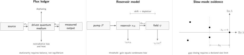
A driven-dissipative claim needs three linked records: the physical flux boundary, any reservoir reduction used in modeling, and the slow mode whose scaling supports a transition. Stationary output establishes balance; it does not by itself establish equilibrium or a thermodynamic phase.

A minimal birth–death mode

Consider a bosonic mode with incoherent single-particle pump $P$ and loss $\kappa$:

$$\dot\rho = -\frac{i}{\hbar}[H,\rho] + P\mathcal D[a^\dagger]\rho + \kappa\mathcal D[a]\rho,$$

where

$$\mathcal D[L]\rho = L\rho L^\dagger - \frac{1}{2} \left\{ L^\dagger L,\rho \right\}.$$

For $n=a^\dagger a$,

$$\frac{d}{dt}\langle n\rangle = P\left( \langle n\rangle+1 \right) - \kappa\langle n\rangle.$$

If $P<\kappa$, the stationary occupation is

$$\langle n\rangle_{\mathrm{ss}} = \frac{P}{\kappa-P}.$$

The divergence at $P=\kappa$ is not a prediction of infinite laboratory intensity. It says the linear model has omitted saturation, nonlinear loss, pump depletion, interactions, or another stabilizing process. Threshold models should identify which omitted mechanism regularizes growth.

Exciton–Polaritons

Exciton–polaritons are hybrid light–matter quasiparticles formed when a confined photon mode and an exciton remain in the strong-coupling regime. For one in-plane momentum, a simple coupled-mode Hamiltonian is

$$H_{\mathrm{xc}} = \begin{pmatrix} E_C & g \\ g & E_X \end{pmatrix},$$

with eigenenergies

$$E_{\pm} = \frac{E_C+E_X}{2} \pm \frac{1}{2} \sqrt{ \left( E_C-E_X \right)^2 +4g^2 }.$$

The anticrossing and linewidths must demonstrate that the hybrid branches remain resolved in the regime being discussed. At high density, screening, phase-space filling, heating, or other nonlinearities can weaken strong coupling and permit an ordinary photon-lasing regime. Calling all coherent microcavity emission “polariton condensation” erases this distinction.

Polaritons combine a small photon-derived effective mass with exciton-derived interactions, but they also inherit radiative loss. A sustained population therefore requires pumping. Nonresonant pumping commonly creates an excitonic reservoir that relaxes into lower-polariton states; resonant pumping instead injects a selected polariton mode with a controlled phase and momentum. These protocols realize different symmetries and different fluctuation problems.

Open-dissipative Gross–Pitaevskii model

A widely used mean-field reduction for a nonresonantly pumped scalar condensate couples a complex polariton field $\psi(\mathbf r,t)$ to a reservoir density $n_R(\mathbf r,t)$:

$$\begin{aligned} i\hbar\partial_t\psi ={}& \left[ -\frac{\hbar^2\nabla^2}{2m} +V(\mathbf r) +g_C\lvert\psi\rvert^2 +g_R n_R \right]\psi \\ &+ \frac{i\hbar}{2} \left( R n_R-\gamma_C \right)\psi, \\ \partial_t n_R ={}& P(\mathbf r,t) - \left( \gamma_R+R\lvert\psi\rvert^2 \right)n_R. \end{aligned}$$

$m$ is the lower-polariton mass, $g_C$ is the condensate interaction, $g_R$ is the reservoir-induced shift, $R$ is the stimulated scattering coefficient, and $\gamma_C,\gamma_R$ are condensate and reservoir loss rates. The imaginary term is gain minus loss; it is not an imaginary conservative potential.

For a homogeneous, time-independent pump and a stable uniform solution, the below-threshold reservoir is $n_R=P/\gamma_R$. Linear gain begins when

$$R n_R=\gamma_C,$$

so the mean-field threshold is

$$P_{\mathrm{th}} = \frac{\gamma_C\gamma_R}{R}.$$

Above threshold, the idealized steady solution clamps the reservoir and grows the condensate:

$$\begin{aligned} n_R^{\mathrm{ss}} &= \frac{\gamma_C}{R}, \\ \lvert\psi_{\mathrm{ss}}\rvert^2 &= \frac{ P-P_{\mathrm{th}} }{ \gamma_C }. \end{aligned}$$

These formulas are useful checks, not universal fits. A finite spot introduces outward flow and boundaries; multiple reservoirs introduce extra relaxation clocks; spin introduces coupled polarization fields; disorder localizes modes; energy-dependent gain selects frequencies; and fluctuations become essential near threshold and in low dimensions.

What the mean-field model does not certify

The reservoir model can reproduce thresholds, density profiles, blueshifts, collective modes, and instabilities. By itself it does not establish:

• the microscopic value or density dependence of an interaction constant;
• quantum rather than classical fluctuations;
• thermalization to a Bose distribution;
• a unique condensate mode in an inhomogeneous sample;
• long-range order in an infinite low-dimensional system;
• superfluidity from a bright low-momentum peak;
• a universality class without correlation-function scaling.

Parameter inference should use held-out observables. A fit to intensity should predict, for example, the reservoir-induced blueshift, linewidth, spatial flow, response spectrum, or correlation time without retuning every parameter.

Condensation, Lasing, and Superfluidity

A threshold and a narrow line are shared by several coherent emitters. Stronger identification uses a bundle of observables.

Claim	Minimum useful evidence	Important control
polariton branch	resolved strong-coupling dispersion and composition	density-dependent loss of strong coupling
macroscopic occupation	calibrated occupation concentrated in one or a few modes	detector response and collection cone
spontaneous coherence	growth of $g^{(1)}$ without a phase-imprinting source	pump coherence leakage
number statistics	measured $g^{(2)}(0)$ and its pump dependence	timing resolution and background
condensation	occupation, coherence, distribution, and symmetry-consistent onset	photon-lasing crossover
superfluid response	suppressed drag or scattering, critical flow, stiffness, or quantized circulation	density change and finite lifetime

First-order coherence can be written

$$g^{(1)}(\mathbf r,\mathbf r';\tau) = \frac{ \left\langle \psi^\dagger(\mathbf r,t) \psi(\mathbf r',t+\tau) \right\rangle }{ \sqrt{ n(\mathbf r)n(\mathbf r') } },$$

while intensity correlations use

$$g^{(2)}(0) = \frac{ \left\langle a^\dagger a^\dagger aa \right\rangle }{ \langle a^\dagger a\rangle^2 }.$$

Interferometry measures spatial or temporal coherence only after accounting for finite resolution, phase drift, and multimode emission. A value $g^{(2)}(0)\approx1$ is consistent with coherent statistics, but it does not identify the microscopic gain mechanism.

Kasprzak and collaborators combined low-momentum occupation, temporal coherence, long-range spatial coherence, and polarization in their evidence for polariton condensation. Amo and collaborators tested fluid response by comparing defect scattering below and above the sound-speed scale. Those are different claims: condensation does not automatically imply superfluidity, and suppressed scattering should be checked against trivial changes in density, linewidth, or defect coupling.

Driven condensates can also have universal fluctuations with no equilibrium counterpart. In a suitable one-dimensional polariton lattice, Fontaine and collaborators measured spatiotemporal coherence scaling consistent with Kardar–Parisi–Zhang universality. Such a claim requires scaling functions or exponents over controlled windows, not merely a rough phase profile.

Platform Ledger

Driven-dissipative matter includes natural materials and synthetic lattices of photons, polaritons, atoms, and superconducting modes.

Platform	Controlled input and loss	Direct observables	Dominant inference risk
semiconductor polaritons	optical pump, radiative decay, reservoir relaxation	angle-resolved emission, interferometry, spectra, correlations	heating and crossover to weak coupling
nonlinear photonic resonators	coherent laser drive and photon leakage	homodyne field, transmission, $g^{(2)}$, switching	classical technical noise mistaken for quantum criticality
circuit-QED lattices	microwave drive, port loss, qubit relaxation	complex transmission, emitted spectrum, time traces	disorder, finite size, and readout bandwidth
atoms in optical cavities	transverse or axial pumping, cavity leakage, atomic loss	leaked light, atomic momentum, density order	adiabatic elimination and atom-number drift

The output is not a passive photograph of an isolated state. In a one-sided Markovian port,

$$a_{\mathrm{out}}(t) = a_{\mathrm{in}}(t) - \sqrt{\kappa_{\mathrm{ext}}}\,a(t),$$

up to the declared phase convention. The measured field contains interference between prompt input and cavity emission. Intracavity occupation cannot therefore be inferred from transmitted intensity without an input–output calibration.

Open-System Phase Transitions

For a time-independent Markovian model,

$$\dot\rho=\mathcal L\rho.$$

Let right eigenoperators obey

$$\mathcal L R_j = \lambda_j R_j, \qquad \lambda_0=0.$$

When the steady state is unique and the remaining modes decay, a common spectral gap is

$$\Delta_{\mathcal L} = -\max_{j\ne0} \operatorname{Re}\lambda_j.$$

The generic definitions and nonnormality cautions belong to Steady States and Relaxation. For material claims, the key point is operational: a small gap produces a long relaxation or switching time, but a single long time at one device size does not establish gap closure.

Finite systems and singular limits

For a finite-dimensional, smoothly parameterized generator with a unique isolated steady state, observables are generally analytic until a spectral degeneracy is encountered. Sharp nonanalytic phase behavior ordinarily requires a declared singular limit. That limit may be:

• the number of lattice sites $L\to\infty$;
• a large occupation or weak-noise limit;
• increasing atom number or cooperativity;
• a mode-volume scaling that keeps nonlinear energy extensive;
• a continuum or long-wavelength limit.

The scaling prescription is part of the phase definition. Increasing drive power alone is not automatically a thermodynamic limit, because it can also change heating, saturation, microscopic parameters, and the number of active modes.

Near a first-order dissipative transition, a finite system can show a bimodal field distribution and rare switching between dim and bright metastable states. The stationary mean then lies between two values that no single trajectory occupies for long. Histograms and dwell-time distributions are more informative than the mean.

Why hysteresis is not enough

Hysteresis can result from true multistability, metastable switching, a slow reservoir, a detector filter, thermal drift, or a sweep that outruns relaxation. Its area depends on the sweep protocol. A defensible transition analysis reports:

1. upward and downward sweep rates and waiting times;
2. stationary time traces at fixed control values;
3. switching distributions or the slowest relaxation time;
4. noise and drift controls;
5. a declared size parameter and scaling trend;
6. an order parameter or distribution linked to a model.

Rodriguez and collaborators measured sweep-time dependence of optical hysteresis in a semiconductor microcavity. Fitzpatrick and collaborators observed bistability and long switching times in a 72-site circuit-QED lattice. Fink and collaborators resolved bimodal phase-space distributions across photon-blockade breakdown. These experiments expose complementary parts of the evidence ladder; none makes hysteresis a universal proxy for a phase transition.

An accepted 2026 PRX Quantum paper by Castillo-Moreno and collaborators reports a multimode dim-to-bright transition in a 21-resonator superconducting Bose–Hubbard simulator, with measured switching times from milliseconds to $143\,\mathrm{s}$. Its accepted-paper status, finite size, and model range should remain explicit until a version of record and broader scaling evidence are available.

Evidence ladder

A strong dissipative-transition claim assembles progressively harder tests:

Level	Evidence
response	reproducible change in a calibrated steady observable
fluctuations	full distributions, $g^{(2)}$, susceptibility, or switching statistics
dynamics	critical slowing, a soft mode, or Liouvillian-gap proxy
structure	spatial correlations, order parameter, symmetry, or mode-resolved reorganization
scaling	finite-size or controlled weak-noise scaling with corrections
universality	multiple exponents or scaling functions and competing-class exclusions

A laser threshold, a dissipative phase transition, a dynamical instability, and an exceptional point are not synonyms. A laser threshold concerns gain, loss, and coherence onset. A dissipative transition concerns a singular change of the stationary state in a declared limit. An instability concerns linearized dynamics around a solution. An exceptional point concerns eigenvalue and eigenvector coalescence of a non-Hermitian operator; its canonical treatment belongs to Open Quantum Materials.

Choosing Lindblad or Keldysh

A Lindblad equation and a Schwinger–Keldysh field theory are not rival labels for the same approximation. They answer different scales of question.

Need	Natural starting point
few modes, trajectories, counting statistics, exact positivity	Lindblad master equation
calibrated Markovian ports and finite-size spectra	Lindblad plus input–output theory
collective fields, response and noise, long wavelengths	Schwinger–Keldysh action
colored reservoirs or memory kernels	influence functional or non-Markovian method
critical exponents and renormalization	Keldysh field theory and RG

Under the convention

$$\begin{aligned} G^R(t) &= -i\theta(t) \left\langle [\phi(t),\phi(0)] \right\rangle, \\ G^K(t) &= -i \left\langle \{\phi(t),\phi(0)\} \right\rangle, \end{aligned}$$

thermal equilibrium imposes the bosonic fluctuation–dissipation relation

$$G^K(\omega) = \coth\!\left( \frac{\hbar\omega}{2k_B T} \right) \left[ G^R(\omega)-G^A(\omega) \right].$$

A driven steady state generally has independent response and noise sectors. Fitting one low-frequency ratio by an effective temperature does not prove a global Gibbs state; the inferred temperature may depend on frequency, momentum, and observable. Schwinger–Keldysh Bridge owns the contour construction, Green-function conventions, influence functionals, and consistency constraints.

Experimental Workflow

1. Declare the boundary. List retained modes, reservoirs, ports, and unmeasured sinks.
2. Calibrate input and output. Convert source settings and detector counts to fluxes with uncertainty.
3. Resolve clocks. Compare drive, loss, dephasing, reservoir, switching, sweep, and acquisition times.
4. Test stationarity. Use fixed-parameter time traces, not only scans.
5. Measure distributions. Means can conceal multimodality, intermittency, and phase diffusion.
6. Validate the model out of sample. Fit one subset of observables and predict another.
7. State the limit. Identify the effective size and how parameters scale with it.
8. Use the narrowest claim. Report crossover, metastability, critical scaling, or phase transition according to the evidence actually obtained.

Common Mistakes

• Treating a steady state as an equilibrium state because its mean observables stop changing.
• Reporting pump power without absorbed flux, spot size, spectral width, or coupling efficiency.
• Calling a linewidth collapse sufficient evidence for condensation or superfluidity.
• Ignoring the loss of strong coupling at high excitation density.
• Inferring intracavity occupation directly from transmission without prompt-field interference.
• Using a deterministic Gross–Pitaevskii equation to make claims about quantum fluctuations.
• Calling any S-shaped response a first-order phase transition.
• Extracting a “Liouvillian gap” from one exponential fit without checking observable overlap or multiple slow modes.
• Treating a no-jump non-Hermitian Hamiltonian as the unconditional open-system dynamics.
• Assigning one effective temperature to a driven state without testing fluctuation–dissipation consistency.

Exercises

1. Linear pump threshold

For the birth–death mode with pump $P$ and loss $\kappa$, solve the equation for $\langle n(t)\rangle$ from an initial value $n_0$. Explain what changes at $P=\kappa$.

Solution

For $P\ne\kappa$,

$$\langle n(t)\rangle = \frac{P}{\kappa-P} + \left( n_0-\frac{P}{\kappa-P} \right) e^{-(\kappa-P)t}.$$

For $P<\kappa$, the mode relaxes to $P/(\kappa-P)$. At $P=\kappa$, the rate equation becomes $\dot n=P$, so occupation grows linearly. For $P>\kappa$, it grows exponentially. The latter regimes reveal the absence of saturation or nonlinear loss in the model; they do not predict an indefinitely growing real device.

2. Reservoir threshold and clamping

For the homogeneous open-dissipative Gross–Pitaevskii equations, derive $P_{\mathrm{th}}$, $n_R^{\mathrm{ss}}$, and $\lvert\psi_{\mathrm{ss}}\rvert^2$ above threshold.

Solution

Below threshold, $\psi=0$ and stationarity gives $n_R=P/\gamma_R$. The field becomes marginal when $Rn_R=\gamma_C$, hence

$$P_{\mathrm{th}} = \frac{\gamma_C\gamma_R}{R}.$$

For a nonzero stationary condensate, gain balance fixes $n_R^{\mathrm{ss}}=\gamma_C/R$. The reservoir equation then gives

$$P = \left( \gamma_R+R\lvert\psi_{\mathrm{ss}}\rvert^2 \right) \frac{\gamma_C}{R},$$

and therefore

$$\lvert\psi_{\mathrm{ss}}\rvert^2 = \frac{P-P_{\mathrm{th}}}{\gamma_C}.$$

The clamping is a property of this homogeneous mean-field reduction, not a universal microscopic law.

3. Close a flux ledger

A device absorbs $12.0\,\mathrm{nW}$ from a pump. Calibrated radiative output is $7.1\,\mathrm{nW}$ and nonradiative recombination carries $2.6\,\mathrm{nW}$. In a stationary state, what residual power must leave through other channels? What uncertainty is missing from this calculation?

Solution

Stationarity requires

$$P_{\mathrm{other}} = 12.0-7.1-2.6 = 2.3\,\mathrm{nW}.$$

The arithmetic does not establish significance without uncertainties and covariance for absorbed power, collection efficiency, spectral integration, and nonradiative inference. A mismatch smaller than the propagated calibration uncertainty would not resolve an additional channel.

4. Gap-scaling audit

Suppose the slowest measured relaxation rates for effective sizes $L=8,12,16$ are $0.090,0.043,0.026$ in the same units. Is this enough to claim $\Delta_{\mathcal L}\to0$?

Solution

No. The downward trend is consistent with a closing gap, but three sizes do not distinguish a power law, exponential closing, crossover, or nonzero asymptote. One must define how all microscopic parameters scale with $L$, estimate uncertainties, check that the measured observable overlaps the slow mode, test additional sizes, and compare competing finite-size forms. Direct switching statistics or independent spectroscopy of the slow mode would strengthen the inference.

5. Dynamic hysteresis

An optical cavity shows a wide hysteresis loop for a fast frequency sweep and a much narrower loop when the sweep is slowed. Give two interpretations and one measurement that helps distinguish them.

Solution

The loop can reflect metastable switching near a first-order dissipative transition, or it can be a purely dynamic lag caused by a reservoir, thermal drift, or detector response. Holding the control parameter fixed inside the loop and recording long time traces tests for stationary bimodality and stochastic switching. Varying the hold time, sweep time, and detector bandwidth helps separate intrinsic switching from instrumental lag.

6. Condensation versus photon lasing

A microcavity develops a sharp intensity threshold, a narrow emission line, and $g^{(2)}(0)\approx1$. What additional observations are needed before identifying a polariton condensate?

Solution

Those three observations demonstrate coherent emission but are shared by photon lasers. The experiment should verify resolved strong coupling and lower-polariton dispersion at the operating density, calibrate mode occupation, measure spatial or temporal coherence without phase leakage from the pump, and monitor the density-dependent crossover toward weak coupling. Population distribution, polarization, blueshift, and reservoir behavior provide further controls. Superfluidity would require an additional response measurement such as defect scattering, drag, stiffness, or circulation.

Research Status

The existence of driven nonequilibrium steady states, polariton condensation, input–output relations, and dissipative critical phenomena is standard. The universality and thermodynamic interpretation of particular platforms remain active because finite size, long switching times, technical noise, reservoir memory, and model reduction can imitate or obscure asymptotic behavior.

Current frontiers include:

• multimode and spatially extended dissipative transitions with controlled scaling;
• quantum rather than semiclassical fluctuation regimes;
• driven condensate universality beyond mean field;
• simultaneous reconstruction of response, noise, and entropy production;
• reservoir-aware state preparation and stabilization;
• interfaces between topological, strongly correlated, and dissipative photonic matter.

Connections

• Artificial Lattices and Designer Matter compares photonic, polaritonic, and circuit arrays with nominally closed simulator platforms and makes pump, loss, and detector contracts explicit.
• Driven Many-Body Systems — extensive forcing, heating, and cycle balance.
• Driven Open Systems — time-dependent master equations and rotating frames.
• Steady States and Relaxation — kernels, Liouvillian spectra, dark states, and metastability.
• Input–Output Theory — traveling fields and calibrated ports.
• Schwinger–Keldysh Bridge — response, fluctuations, influence functionals, and nonequilibrium field theory.
• Reservoir Engineering — dissipation deliberately designed to stabilize target states.
• Bose–Einstein Condensation — equilibrium condensation and thermodynamic-limit baseline.
• Cavity QED — coherent light–matter coupling and strong-coupling diagnostics.
• Open Quantum Materials — environmental self-energies, non-Hermitian models, exceptional points, and boundary-sensitive spectra.

References

• I. Carusotto and C. Ciuti, “Quantum fluids of light,” Reviews of Modern Physics 85, 299–366 (2013).
• H. Deng, H. Haug, and Y. Yamamoto, “Exciton-polariton Bose–Einstein condensation,” Reviews of Modern Physics 82, 1489–1537 (2010).
• J. Kasprzak, M. Richard, S. Kundermann, et al., “Bose–Einstein condensation of exciton polaritons,” Nature 443, 409–414 (2006).
• M. H. Szymańska, J. Keeling, and P. B. Littlewood, “Nonequilibrium quantum condensation in an incoherently pumped dissipative system,” Physical Review Letters 96, 230602 (2006).
• M. Wouters and I. Carusotto, “Excitations in a nonequilibrium Bose–Einstein condensate of exciton polaritons,” Physical Review Letters 99, 140402 (2007).
• A. Amo, J. Lefrère, S. Pigeon, et al., “Superfluidity of polaritons in semiconductor microcavities,” Nature Physics 5, 805–810 (2009).
• Q. Fontaine, D. Squizzato, F. Baboux, et al., “Kardar–Parisi–Zhang universality in a one-dimensional polariton condensate,” Nature 608, 687–691 (2022).
• L. M. Sieberer, M. Buchhold, and S. Diehl, “Keldysh field theory for driven open quantum systems,” Reports on Progress in Physics 79, 096001 (2016).
• M. Fitzpatrick, N. M. Sundaresan, A. C. Y. Li, J. Koch, and A. A. Houck, “Observation of a dissipative phase transition in a one-dimensional circuit QED lattice,” Physical Review X 7, 011016 (2017).
• J. M. Fink, A. Dombi, A. Vukics, A. Wallraff, and P. Domokos, “Observation of the photon-blockade breakdown phase transition,” Physical Review X 7, 011012 (2017).
• S. R. K. Rodriguez, W. Casteels, F. Storme, et al., “Probing a dissipative phase transition via dynamical optical hysteresis,” Physical Review Letters 118, 247402 (2017).
• C. Castillo-Moreno, T. Sépulcre, T. Hillmann, K. R. Amin, M. Kervinen, and S. Gasparinetti, “Experimental observation of multimode quantum phase transitions in a superconducting Bose-Hubbard simulator,” PRX Quantum, accepted 24 June 2026.
• F. Minganti, A. Biella, N. Bartolo, and C. Ciuti, “Spectral theory of Liouvillians for dissipative phase transitions,” Physical Review A 98, 042118 (2018).
• W. Casteels, R. Fazio, and C. Ciuti, “Critical dynamical properties of a first-order dissipative phase transition,” Physical Review A 95, 012128 (2017).
• S. Diehl, A. Micheli, A. Kantian, B. Kraus, H.-P. Büchler, and P. Zoller, “Quantum states and phases in driven open quantum systems with cold atoms,” Nature Physics 4, 878–883 (2008).
• K. Baumann, C. Guerlin, F. Brennecke, and T. Esslinger, “Dicke quantum phase transition with a superfluid gas in an optical cavity,” Nature 464, 1301–1306 (2010).
• J. Klinder, H. Keßler, M. Wolke, L. Mathey, and A. Hemmerich, “Dynamical phase transition in the open Dicke model,” Proceedings of the National Academy of Sciences 112, 3290–3295 (2015).
• C. W. Gardiner and M. J. Collett, “Input and output in damped quantum systems: Quantum stochastic differential equations and the master equation,” Physical Review A 31, 3761–3774 (1985).

Summary

Driven-dissipative matter is defined by throughput: sustained sources, losses, reservoirs, and readout select the state together. Polariton fluids make this structure especially visible because hybrid light–matter modes require pumping to survive. Thresholds, coherence, superfluid response, and phase-transition claims require distinct evidence. Liouvillian models resolve finite-mode dynamics and switching; Schwinger–Keldysh methods organize response, noise, and critical fields. In every case, the trustworthy route runs through calibrated fluxes, full distributions, declared limits, and claims no broader than the measurements support.