Floquet Quantum Matter

Floquet quantum matter is matter whose useful dynamical structure is created or reorganized by a drive that repeats over many controlled cycles. The repeated drive can dress bands, renormalize tunneling and exchange, synthesize gauge fields, generate topology tied to an entire cycle, or stabilize long-lived subharmonic response. None of those outcomes follows merely from applying a periodic field. The drive must remain coherent long enough, the target structure must be resolved against broadening and heating, and the measured state must actually occupy the relevant Floquet modes.

This page is the materials-and-experiment bridge. It owns waveform calibration, quasienergy spectroscopy, effective-model validation, platform comparisons, topological evidence ladders, and usable-lifetime budgets. Floquet Systems Preview remains the canonical home for many-body Floquet eigenstate thermalization, heating regimes, time-crystal criteria, and anomalous-unitary theory. Floquet Theorem in Quantum Mechanics owns the exact theorem, while High-Frequency Expansions owns inverse-frequency constructions and truncation control.

From Waveform to Material Claim

An ideal Floquet Hamiltonian obeys strict periodicity. A laboratory drive also has an envelope, loading ramp, phase noise, spatial profile, and finite duration:

$$\begin{gathered} H(t+T)=H(t), \qquad \Omega=\frac{2\pi}{T}, \\ N_{\mathrm{cyc}} = \frac{\tau_{\mathrm{env}}}{T}. \end{gathered}$$

Here $\tau_{\mathrm{env}}$ is the interval over which the drive amplitude is approximately controlled. A quasienergy description is useful only if the system experiences enough phase-coherent cycles for the relevant observable. A ten-cycle pulse can reveal photon-dressed replicas without establishing a long-lived many-body phase.

A complete drive record includes:

Layer	Quantities to report
Carrier	$\Omega$, polarization, phase, harmonics, and timing jitter
Envelope	Turn-on, plateau, turn-off, pulse duration, and shot-to-shot variation
Coupling	Electric field, vector potential, lattice displacement, gate sequence, or spin-rotation angle
Geometry	Beam spot, penetration depth, lattice inhomogeneity, boundaries, and driven volume
State	Initial temperature, filling, symmetry sector, and loading protocol
Environment	Dephasing, particle loss, phonons, substrate, cavity leakage, and measurement backaction
Readout	Probe phase within the cycle, integration window, resolution, and response matrix elements

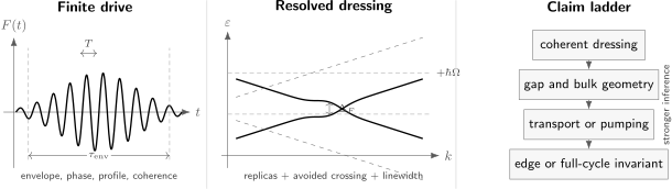
A finite periodic waveform first has to produce resolvable quasienergy dressing. Spectroscopy, dynamics, transport, and boundary response then support progressively stronger claims; no single sideband establishes a Floquet phase.

Calibrating the Drive

For a charged Bloch system coupled through a vector potential, a common starting point is

$$H(\mathbf k,t) = H_0\!\left( \mathbf k-\frac{q}{\hbar}\mathbf A(t) \right).$$

If an approximately monochromatic electric field has amplitude $E_0$, then $A_0\sim E_0/\Omega$. A natural bond-scale drive strength is

$$\kappa = \frac{\lvert q\rvert aE_0}{\hbar\Omega},$$

where $a$ is the relevant hopping distance. Reporting only intensity hides the frequency dependence of $\kappa$. It also hides local-field corrections, screening, and polarization relative to crystal axes.

Optical-lattice shaking is often calibrated by displacement or inertial force rather than electric field. Digital spin and qubit experiments instead need pulse angles, gate order, coherent over-rotation, and idle evolution. These controls are not interchangeable, even when their leading effective Hamiltonians look alike.

The drive frequency must be compared with several scales:

• target bandwidths, gaps, interactions, and exchange energies;
• unwanted interband gaps and higher orbital levels;
• linewidths and dephasing rates;
• bath and phonon frequencies;
• the inverse ramp time and pulse bandwidth.

“High frequency” means high relative to the local processes retained in a declared model. It need not be high relative to every microscopic transition. Near-resonant engineering deliberately violates an off-resonant condition and therefore requires explicit leakage and occupation measurements.

Quasienergy as a Laboratory Observable

Floquet quasienergy is defined modulo the drive quantum. In an extended-zone picture, a dressed band appears as replicas

$$\varepsilon_{\alpha m}(\mathbf k) = \varepsilon_\alpha(\mathbf k) +m\hbar\Omega, \qquad m\in\mathbb Z.$$

Where replicas hybridize, a drive-induced avoided crossing can open. A finite pulse resolves a gap $\Delta_F$ only if it exceeds intrinsic broadening, instrumental resolution, and the Fourier width of the drive. A useful heuristic is

$$\Delta_F \gtrsim \left[ \Gamma^2 +\delta E_{\mathrm{inst}}^2 +\left( \frac{\hbar}{\tau_{\mathrm{env}}} \right)^2 \right]^{1/2}.$$

This is a resolution budget, not a universal theorem. Different line shapes combine differently, and a probe may broaden energy while improving time resolution.

Time-resolved photoemission

Time- and angle-resolved photoemission does not directly photograph a quasienergy eigenvalue. Its intensity is schematically a probe-windowed two-time correlator:

$$\begin{aligned} I(\mathbf k,\omega;t_d) &\propto \int dt\,dt'\, s(t-t_d)s(t'-t_d) \\ &\quad\times e^{i\omega(t-t')} G^<_{\mathbf k}(t,t'). \end{aligned}$$

The pulse envelope $s$, photoemission matrix elements, occupations, and final-state propagation all matter. A free photoelectron can itself be dressed by the pump, producing Volkov sidebands that resemble initial-state Floquet replicas. Floquet and Volkov pathways can also interfere.

Therefore a sideband claim should include:

1. polarization and incidence-angle controls that change final-state dressing;
2. momentum-resolved comparison with both Floquet and Volkov calculations;
3. delay dependence through and beyond pump–probe overlap;
4. field-strength and frequency scaling;
5. an avoided crossing or another coherent-hybridization signature when resolution permits;
6. linewidth and dephasing estimates.

The 2025 graphene measurements separated these pathways using momentum and polarization structure. The 2026 observation of an avoided-crossing gap added a stronger coherent-band-engineering signature. Neither result by itself proves a topological steady state or quantized transport.

Cold-atom and synthetic platforms

Ultracold atoms do not provide electronic photoemission, but band mapping, state tomography, center-of-mass drift, circular dichroism, and quench dynamics can reconstruct quasienergy gaps and Berry-curvature information. The absence of a filled electronic Fermi sea is an advantage for state preparation but makes the measured response preparation dependent.

Photonic and acoustic platforms can image propagation and edge transport with exceptional spatial resolution. In many such systems a propagation coordinate plays the role of time. This faithfully tests a wave equation and its unitary topology, but it does not reproduce fermionic occupations, quantum thermalization, or energy absorption by an isolated many-body state.

Inferring an Effective Hamiltonian

An effective Hamiltonian is an experimentally tested model, not the logarithm of one fitted cycle presented as a material property. Its validity depends on the stroboscopic phase, branch choice, ramp, state, observable, and time window.

For a family of observables $O_a$, a useful validation residual is

$$\chi_{\mathrm{eff}}^2 = \sum_{a,n,\tau} \frac{ \left[ O_a^{\mathrm{data}}(nT+\tau) -O_a^{\mathrm{eff}}(nT+\tau) \right]^2 }{ \sigma_{a,n,\tau}^2 }.$$

The sum should include held-out observables and at least two phases $\tau$ within the cycle. A model that fits only stroboscopic populations may fail for currents or micromotion. Likewise, matching a gap does not validate the predicted occupations.

A strong inference workflow compares:

• the measured waveform with an exact finite-drive calculation;
• the exact calculation with the truncated effective model;
• bare observables with their micromotion-dressed counterparts;
• multiple frequencies and amplitudes with one shared parameter set;
• the driven system with a static benchmark having matched effective couplings;
• retained-band predictions with measured leakage into excluded bands.

Near a multiphoton resonance, denominators in an off-resonant expansion become small. The resonant states must then enter the explicit model. Calling the resulting fit “high-frequency Floquet engineering” obscures the mechanism.

Platform Ledger

Platform	Typical periodic control	Strongest direct evidence	Principal limitation
Electronic solids	Mid-infrared, terahertz, or optical field	Time-resolved spectra, ultrafast current, diffraction, polarization dependence	Short coherence, nonequilibrium occupations, depth mismatch, phonons
Optical lattices	Shaking, modulation, Raman-assisted hopping	Band mapping, Berry-curvature drift, correlations, heating and loss	Higher bands, trap inhomogeneity, finite loading
Trapped ions and qubits	Pulse sequences or programmed gates	Site-resolved dynamics, tomography, subharmonic rigidity	Finite size, calibration drift, decoherence
Photonic or acoustic lattices	Spatial or temporal modulation	Edge propagation, scattering around defects, field reconstruction	Wave analogue rather than thermal quantum matter

The right conclusion is platform specific. A photonic edge mode can establish anomalous unitary topology without answering a heating question. A cold-atom heating curve can test prethermal scaling without demonstrating an electronic material. A solid-state Hall pulse can reveal a helicity-dependent transverse response while still requiring a model of carriers, contacts, and dissipation.

Floquet Topology: An Evidence Ladder

Periodic driving supports two distinct topological strategies:

1. engineer a static-looking effective band Hamiltonian with familiar Chern or symmetry invariants;
2. realize topology of the full evolution over a cycle, including anomalous edge modes not determined by Floquet-band Chern numbers alone.

Chern Numbers in Band Theory owns static band invariants. Bulk–Boundary Correspondence explains why boundary claims require a specified gap and interface. For a driven system, the evidentiary levels are:

Level	Observation	Supported claim	What remains open
Dressing	Replicas or coherent oscillations	Periodic light–matter or control coupling	Gap, topology, occupation
Hybridization	Resolved avoided crossing with drive scaling	Floquet band formation	Global invariant and response
Bulk geometry	Berry-curvature map, dichroism, or transverse drift	Topology-sensitive band structure	Occupation and boundary transport
Response	Helicity-dependent Hall current or quantized pump	Driven transverse transport	Separation from photocarriers, baths, contacts
Boundary	Gap-resolved chiral edge propagation	Driven bulk–boundary relation	Many-body stability and heating
Full-cycle anomaly	Gap invariants plus edge modes despite vanishing band Chern numbers	Anomalous Floquet topology	Interaction and thermodynamic stability

Even for a noninteracting Floquet band, Hall response depends on occupations. Schematically in two dimensions,

$$\sigma_{xy}^{\mathrm{band}} = -\frac{q^2}{\hbar} \sum_\alpha \int_{\mathrm{BZ}} \frac{d^2k}{(2\pi)^2} f_\alpha(\mathbf k) \Omega_\alpha^F(\mathbf k).$$

A nonthermal $f_\alpha(\mathbf k)$ generally prevents quantization even when the quasienergy band has a nonzero Chern number. Micromotion, contacts, and baths can contribute additional terms. Thus “topological band” and “quantized topological transport” are different claims.

The shaken-lattice Haldane experiment combined gap closing with Berry-curvature-sensitive drift. Later cold-atom work inferred anomalous Floquet invariants using gap measurements and local Hall deflections. Photonic lattices directly imaged robust edge propagation. These are complementary tests, not interchangeable demonstrations of one universal phase.

Heating, Dephasing, and the Usable Window

The operational lifetime is set by the first process that destroys the intended description:

$$\tau_{\mathrm{use}} = \min \left( \tau_\phi, \tau_{\mathrm{heat}}, \tau_{\mathrm{loss}}, \tau_{\mathrm{env}}, \tau_{\mathrm{drift}} \right).$$

For an engineered gap or coupling $\Delta_{\mathrm{eng}}$, define

$$Q_F = \frac{ \Delta_{\mathrm{eng}}\tau_{\mathrm{use}} }{\hbar}.$$

A value $Q_F\lesssim 1$ means the target dynamics cannot complete even one characteristic evolution before the description fails. A larger value is necessary, but not sufficient, for useful Floquet matter.

In bounded, nearly isolated lattice models, generic periodic driving can lead toward sector-constrained infinite-temperature local behavior. At high local frequency, absorption can be exponentially slow and a prethermal effective Hamiltonian can govern a long interval. Prethermalization Preview owns the plateau and escape criteria.

Real materials are not closed bounded spin systems. Electrons exchange energy with phonons, substrates, leads, and photons. Dissipation may destroy coherence, remove entropy, or stabilize a periodic nonequilibrium state. The correct question is not simply “does it heat?” but:

• where does the absorbed energy go;
• which subsystem remains coherent;
• whether the occupation is stationary, periodic, or drifting;
• whether loss selectively removes high-energy particles;
• whether the engineered response outlives loading and measurement.

In optical lattices, atom loss can cool the particles that remain, so temperature and retained energy alone can understate absorption. In solids, an apparently steady signal during a pump envelope can reflect balance among absorption, scattering, and escape rather than an isolated Floquet eigenstate. Driven Many-Body Systems owns the power ledger, and Driven Open Systems owns periodic reduced-state dynamics.

Time Crystals: Cross-Link, Not Shortcut

A discrete time crystal responds with a robust integer multiple of the drive period. A subharmonic Fourier peak is only the beginning. Interaction dependence, frequency locking over a parameter interval, lifetime scaling, spatial correlations, and exclusion of beating or pulse errors are required.

This page does not duplicate the phase criteria. Floquet Systems Preview owns localized and prethermal stabilization, quasienergy pairing, finite-size discipline, and the experimental claim test. In a materials context, the key addition is to include drive inhomogeneity, readout aliasing, and open-system synchronization among the alternative explanations.

Status as of 2026

Established within controlled platforms

• Periodic modulation can engineer tunneling, gauge fields, magnetic exchange, and topological band structure over finite windows.
• Floquet–Bloch replicas and hybridization gaps have been resolved in selected solid-state systems.
• Cold-atom experiments have reconstructed Berry-curvature information, realized effective Haldane bands, and accessed anomalous Floquet topology.
• Frequency-dependent suppression of many-body heating and prethermal windows has been measured in optical lattices.
• Photonic systems have directly imaged robust ordinary and anomalous Floquet edge transport.

Requires claim-specific qualification

• A measured sideband can include Volkov final-state dressing.
• A light-induced gap need not be topological.
• A topological quasienergy band need not be favorably occupied.
• A Hall pulse need not be quantized or exclusively geometric.
• A prethermal plateau is finite-lived and can be cut short by loss or decoherence.
• A subharmonic response need not be a time-crystalline phase.

Active frontier

• robust interacting Floquet topology in realistic electronic materials;
• simultaneous control of coherence, occupation, heating, and dissipation;
• scalable full-cycle invariants in interacting systems;
• predictive ab initio treatment of driven correlated materials;
• device operation that exploits a Floquet state for many coherent cycles.

Reproducibility Workflow

1. Publish the full waveform, envelope, phase, polarization, and spatial profile.
2. State the microscopic and effective Hilbert spaces, including excluded bands.
3. Report $\Omega/J$, resonant detunings, $\kappa$, and all relevant linewidths.
4. Measure coherent cycle count, heating, loss, and dephasing independently.
5. Resolve both stroboscopic evolution and at least one intracycle observable.
6. Separate state dressing from probe or final-state dressing.
7. Validate an effective Hamiltonian on held-out observables and parameter sweeps.
8. Measure occupations as well as quasienergy structure.
9. Match each topology claim to bulk, response, boundary, or full-cycle evidence.
10. State the finite time and size over which the claim is supported.

Common Mistakes

• Treating a finite pulse as an infinitely periodic Hamiltonian.
• Reporting intensity without the field, frequency, polarization, and local coupling.
• Calling every photon replica a Floquet–Bloch state.
• Ignoring Volkov sidebands in photoemission.
• Equating a matrix logarithm with a local material Hamiltonian.
• Fitting one stroboscopic observable and ignoring micromotion.
• Inferring a Chern response without measuring occupations.
• Calling a light-induced spectral gap topological without a topology-sensitive probe.
• Treating atom loss as absence of heating.
• Applying isolated-system infinite-temperature language directly to a dissipative solid.
• Calling a subharmonic peak a time crystal.
• Comparing platforms without stating which physical role their time coordinate plays.

Exercises

1. Can the pulse resolve the gap?

A graphene experiment uses $\hbar\Omega=0.20\ \mathrm{eV}$ and a nearly flat drive envelope of duration $\tau_{\mathrm{env}}=300\ \mathrm{fs}$. The intrinsic linewidth is $12\ \mathrm{meV}$, the instrumental energy resolution is $8\ \mathrm{meV}$, and the predicted avoided-crossing gap is $20\ \mathrm{meV}$. Estimate the number of cycles and the resolution budget. Use $\hbar=0.658\ \mathrm{eV\,fs}$.

Solution

The period is

$$T = \frac{2\pi\hbar}{\hbar\Omega} = \frac{ 2\pi(0.658\ \mathrm{eV\,fs}) }{ 0.20\ \mathrm{eV} } \approx 20.7\ \mathrm{fs}.$$

Therefore

$$N_{\mathrm{cyc}} \approx \frac{300}{20.7} \approx 14.5.$$

The Fourier contribution is

$$\frac{\hbar}{\tau_{\mathrm{env}}} \approx 2.2\ \mathrm{meV}.$$

Using the heuristic quadrature budget,

$$\delta E_{\mathrm{tot}} \approx \sqrt{ (12\ \mathrm{meV})^2 +(8\ \mathrm{meV})^2 +(2.2\ \mathrm{meV})^2 } \approx 14.6\ \mathrm{meV}.$$

The predicted $20\ \mathrm{meV}$ gap is larger than this estimate and may be resolvable, but the margin is modest. A line-shape simulation with the actual probe envelope is needed for a quantitative claim.

2. Field amplitude versus Floquet coupling

Two experiments use the same electric-field amplitude $E_0$ and lattice spacing $a$, but experiment B uses half the angular frequency of experiment A. Compare their dimensionless Peierls strengths $\kappa$. Does this prove that B gives better off-resonant engineering?

Solution

Because

$$\kappa = \frac{\lvert q\rvert aE_0}{\hbar\Omega},$$

halving $\Omega$ doubles $\kappa$. This increases the momentum excursion and can strengthen dressing.

It does not establish better off-resonant engineering. The lower frequency may approach intraband, interband, phonon, or many-body resonances; it also narrows the separation between the drive quantum and local energy scales. Leakage and absorption can therefore increase even while $\kappa$ becomes larger.

3. Distinguish Floquet and Volkov sidebands

A time-resolved photoemission spectrum shows replicas separated by $\hbar\Omega$. Design four controls that distinguish initial-state Floquet dressing from final-state Volkov dressing.

Solution

Useful controls are:

1. rotate pump polarization relative to the photoelectron detection plane;
2. map the full momentum dependence rather than one energy cut;
3. compare with a calculation containing both initial- and final-state dressing and their interference;
4. search for avoided crossings where replicas hybridize;
5. vary pump–probe delay through temporal overlap;
6. repeat at several fields and frequencies;
7. change probe photon energy or emission geometry to alter final-state coupling.

No one control is universal. The goal is a joint pattern that cannot be reproduced by Volkov dressing alone.

4. Test an effective Hamiltonian without refitting

An effective model is fitted to stroboscopic density data at one frequency. Propose a held-out test that addresses both micromotion and parameter transfer.

Solution

First freeze all fitted parameters. At the original drive setting, measure a current or correlation function at several phases $\tau$ within the cycle and compare it with the model using the properly dressed observable. This tests micromotion.

Then change the frequency while preserving the calibrated dimensionless drive strength and predict the new data without refitting microscopic couplings. A successful model should reproduce several observables and their phase dependence over a declared time window. Failure localized near a resonance indicates that omitted states or resonant processes must enter the model.

5. Audit a topological Hall claim

Circularly polarized light produces a helicity-dependent transverse current and a gap-like spectral feature. List the additional evidence needed before claiming quantized Floquet topological transport.

Solution

The study should determine:

• whether the gap is a coherent Floquet hybridization gap;
• its momentum dependence and relation to the proposed global invariant;
• occupations of the dressed bands;
• longitudinal and transverse contact response;
• separation of Berry-curvature current from asymmetric photocarriers and rectification;
• dependence on chemical potential, helicity, intensity, and frequency;
• heating, dephasing, and bath effects;
• whether the measured value approaches a quantized plateau with controlled corrections;
• boundary transport or another bulk–boundary diagnostic when relevant.

The reported observations support light-induced transverse response and spectral restructuring. Quantized topology is a stronger statement.

6. Compute the usable Floquet window

A driven device has $T=25\ \mathrm{fs}$, $\tau_\phi=180\ \mathrm{fs}$, $\tau_{\mathrm{heat}}=2.5\ \mathrm{ps}$, $\tau_{\mathrm{loss}}=8\ \mathrm{ps}$, and $\tau_{\mathrm{env}}=400\ \mathrm{fs}$. Its engineered gap is $15\ \mathrm{meV}$. Estimate $N_{\mathrm{use}}$ and $Q_F$.

Solution

Dephasing is the shortest timescale, so

$$\tau_{\mathrm{use}} = 180\ \mathrm{fs}, \qquad N_{\mathrm{use}} = \frac{180}{25} = 7.2.$$

Using $\hbar=658\ \mathrm{meV\,fs}$,

$$Q_F = \frac{ (15\ \mathrm{meV})(180\ \mathrm{fs}) }{ 658\ \mathrm{meV\,fs} } \approx 4.1.$$

The drive supports only about seven coherent cycles and roughly four characteristic gap times. Coherent dressing may be observable, but precision transport or asymptotic many-body claims would be poorly supported. Improving the heating time alone would not help because dephasing is already the bottleneck.

Connections

• Quantum Matter Frontiers and Open Problems freezes waveform, preparation, occupation, heating, dephasing, forward-model alternatives, and the usable lifetime before a driven-material observation is promoted to a phase or mechanism claim.
• Floquet Systems Preview is the canonical many-body regime map and owns time-crystal and anomalous-phase criteria.
• Floquet Operators owns reference-phase dependence and logarithm branches.
• Quasienergies develops zone folding and extended Floquet space.
• Floquet–Magnus Expansion derives the phase-dependent one-cycle expansion.
• Prethermalization Preview owns plateau, lifetime, and escape diagnostics.
• Hall Effect fixes transverse-response and sign conventions.
• Spectral Functions owns retarded and lesser spectral conventions.
• Ultrafast Spectroscopy Overview develops pulse resolution and pump–probe measurement logic.

References

1. M. Bukov, L. D’Alessio, and A. Polkovnikov, “Universal High-Frequency Behavior of Periodically Driven Systems: From Dynamical Stabilization to Floquet Engineering,” Advances in Physics 64, 139–226 (2015), doi:10.1080/00018732.2015.1055918. Reviews gauge, micromotion, and high-frequency engineering.
2. A. Eckardt, “Colloquium: Atomic Quantum Gases in Periodically Driven Optical Lattices,” Reviews of Modern Physics 89, 011004 (2017), doi:10.1103/RevModPhys.89.011004. Reviews optical-lattice implementations and limitations.
3. T. Oka and S. Kitamura, “Floquet Engineering of Quantum Materials,” Annual Review of Condensed Matter Physics 10, 387–408 (2019), doi:10.1146/annurev-conmatphys-031218-013423. Reviews ultrafast solid-state Floquet engineering.
4. M. S. Rudner and N. H. Lindner, “Band Structure Engineering and Non-Equilibrium Dynamics in Floquet Topological Insulators,” Nature Reviews Physics 2, 229–244 (2020), doi:10.1038/s42254-020-0170-z. Separates band topology, occupations, heating, and observable response.
5. N. Goldman and J. Dalibard, “Periodically Driven Quantum Systems: Effective Hamiltonians and Engineered Gauge Fields,” Physical Review X 4, 031027 (2014), doi:10.1103/PhysRevX.4.031027. Develops effective Hamiltonians and micromotion for engineered gauge fields.
6. M. S. Rudner, N. H. Lindner, E. Berg, and M. Levin, “Anomalous Edge States and the Bulk–Edge Correspondence for Periodically Driven Two-Dimensional Systems,” Physical Review X 3, 031005 (2013), doi:10.1103/PhysRevX.3.031005. Establishes full-cycle anomalous Floquet topology.
7. Y. H. Wang, H. Steinberg, P. Jarillo-Herrero, and N. Gedik, “Observation of Floquet–Bloch States on the Surface of a Topological Insulator,” Science 342, 453–457 (2013), doi:10.1126/science.1239834. Reports photon-dressed surface bands and avoided crossings.
8. F. Mahmood et al., “Selective Scattering between Floquet–Bloch and Volkov States in a Topological Insulator,” Nature Physics 12, 306–310 (2016), doi:10.1038/nphys3609. Demonstrates the importance of final-state dressing in photoemission.
9. G. Jotzu et al., “Experimental Realization of the Topological Haldane Model with Ultracold Fermions,” Nature 515, 237–240 (2014), doi:10.1038/nature13915. Realizes an effective driven Haldane band in an optical lattice.
10. N. Fläschner et al., “Experimental Reconstruction of the Berry Curvature in a Floquet Bloch Band,” Science 352, 1091–1094 (2016), doi:10.1126/science.aad4568. Extracts momentum-resolved geometric information after periodic driving.
11. K. Wintersperger et al., “Realization of an Anomalous Floquet Topological System with Ultracold Atoms,” Nature Physics 16, 1058–1063 (2020), doi:10.1038/s41567-020-0949-y. Combines gap and local-Hall measurements to infer anomalous invariants.
12. M. C. Rechtsman et al., “Photonic Floquet Topological Insulators,” Nature 496, 196–200 (2013), doi:10.1038/nature12066. Directly images robust photonic edge propagation.
13. F. Görg et al., “Enhancement and Sign Change of Magnetic Correlations in a Driven Quantum Many-Body System,” Nature 553, 481–485 (2018), doi:10.1038/nature25135. Tests driven exchange engineering in a Fermi–Hubbard platform.
14. M. Reitter et al., “Interaction Dependent Heating and Atom Loss in a Periodically Driven Optical Lattice,” Physical Review Letters 119, 200402 (2017), doi:10.1103/PhysRevLett.119.200402. Resolves interaction, interband, heating, and loss channels.
15. A. Rubio-Abadal et al., “Floquet Prethermalization in a Bose–Hubbard System,” Physical Review X 10, 021044 (2020), doi:10.1103/PhysRevX.10.021044. Measures frequency-dependent suppression of heating.
16. J. W. McIver et al., “Light-Induced Anomalous Hall Effect in Graphene,” Nature Physics 16, 38–41 (2020), doi:10.1038/s41567-019-0698-y. Reports an ultrafast helicity-dependent Hall response with model-dependent Floquet interpretation.
17. M. Merboldt et al., “Observation of Floquet States in Graphene,” Nature Physics 21, 1093–1099 (2025), doi:10.1038/s41567-025-02889-7. Separates Floquet, Volkov, and interference fingerprints in momentum microscopy.
18. D. Choi et al., “Observation of Floquet–Bloch States in Monolayer Graphene,” Nature Physics 21, 1100–1105 (2025), doi:10.1038/s41567-025-02888-8. Resolves replica bands and their polarization dependence.
19. F. Wang et al., “Observation of Floquet-Induced Gap in Graphene,” Nature Materials 25, 1140–1145 (2026), doi:10.1038/s41563-026-02549-y. Reports a polarization-tunable avoided-crossing gap with coherent sidebands.
20. J. Zhang et al., “Observation of a Discrete Time Crystal,” Nature 543, 217–220 (2017), doi:10.1038/nature21413. Provides an early trapped-ion realization of robust subharmonic response.

Further Reading

• M. A. Sentef et al., “Theory of Floquet Band Formation and Local Pseudospin Textures in Pump–Probe Photoemission of Graphene,” Nature Communications 6, 7047 (2015), doi:10.1038/ncomms8047. Connects driven pseudospin dynamics to time-resolved spectra.
• D. V. Else, C. Monroe, C. Nayak, and N. Y. Yao, “Discrete Time Crystals,” Annual Review of Condensed Matter Physics 11, 467–499 (2020), doi:10.1146/annurev-conmatphys-031119-050658. Reviews definitions, stabilization mechanisms, and experimental diagnostics.