High-Frequency Expansions

A high-frequency expansion replaces rapid periodic driving by a slowly acting effective Hamiltonian together with a periodic micromotion transformation. It is useful when a Hamiltonian

$$H(t+T)=H(t), \qquad \Omega=\frac{2\pi}{T},$$

contains a drive frequency whose quantum $\hbar\Omega$ is large compared with the energy scales that couple relevant states. The leading approximation is often the period average. Higher orders retain virtual absorption and emission processes through commutators divided by powers of $\hbar\Omega$.

This page is the canonical home for the general inverse-frequency method, especially the van Vleck organization, its relation to Floquet-space block diagonalization, the separation of effective evolution from micromotion, and the prethermal interpretation in local many-body systems. Floquet Theorem in Quantum Mechanics owns the exact theorem. Magnus Expansion owns the general exponential series, while Floquet–Magnus Expansion owns the direct one-period Magnus construction at a chosen drive phase. Driven Many-Body Systems owns the broader absorption ledger and driven–dissipative distinction. Floquet Systems Preview owns the many-body regime map, Floquet ETH, engineering evidence, and emergent periodic phases. Floquet Quantum Matter supplies the materials-facing waveform, spectroscopy, topology, and lifetime evidence ledger.

The phrase high frequency is relational. A large numerical value of $\Omega$ is not enough: one must identify the matrix elements, bandwidths, detunings, local interaction scales, populated energy window, and observation time against which it is large.

Fourier Convention

Use the Fourier decomposition

$$H(t) = \sum_{m\in\mathbb Z} H_m e^{im\Omega t},$$

with

$$H_m = \frac{1}{T} \int_0^T e^{-im\Omega t}H(t)\,dt.$$

Hermiticity of $H(t)$ implies

$$H_{-m}=H_m^\dagger.$$

The zero mode is the period average,

$$H_0 = \frac{1}{T} \int_0^T H(t)\,dt.$$

Fixing the sign in the Fourier exponential is essential. Reversing that convention reverses the order of several commutators. Formulas from different sources should therefore never be combined until their Fourier and micromotion conventions have been translated.

Separation in Extended Floquet Space

Floquet modes solve the quasienergy eigenvalue problem

$$\left( H(t)-i\hbar\partial_t \right) \lvert u_\alpha(t)\rangle = \varepsilon_\alpha \lvert u_\alpha(t)\rangle.$$

It is useful to regard the quasienergy operator

$$\mathcal Q \equiv H(t)-i\hbar\partial_t$$

as a time-independent operator on the extended space of $T$-periodic functions. In the basis

$$\lvert \alpha,m\rangle\!\rangle = \lvert\alpha\rangle e^{im\Omega t},$$

its blocks are

$$\begin{aligned} & \langle\!\langle \alpha',m' \rvert \mathcal Q \lvert \alpha,m \rangle\!\rangle \\ &\quad= \langle\alpha'| H_{m'-m} |\alpha\rangle \\ &\qquad+ \delta_{m'm}\delta_{\alpha'\alpha} m\hbar\Omega. \end{aligned}$$

The diagonal sectors are displaced by $m\hbar\Omega$. A Fourier component $H_r$ couples sectors whose photon labels differ by $r$. The word photon is convenient bookkeeping here; the periodic drive need not be a quantized electromagnetic field.

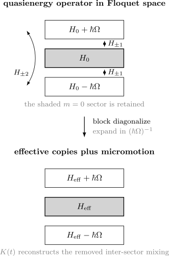
At large $\hbar\Omega$, Fourier harmonics couple well-separated Floquet sectors. The shaded $m=0$ sector is retained. A perturbative block diagonalization produces repeated copies $H_{\mathrm{eff}}+m\hbar\Omega$, while the periodic kick operator $K(t)$ restores the inter-sector admixture as micromotion.

This is an energy-space version of scale separation. Eliminating remote Floquet sectors is closely analogous to a Schrieffer–Wolff Transformation. The large denominators are now multiples of $\hbar\Omega$, and the eliminated admixture reappears as micromotion rather than disappearing from the physical state.

Effective Hamiltonian and Micromotion

A useful exact factorization is

$$U(t,t_0) = e^{-iK(t)} e^{-iH_{\mathrm{eff}}(t-t_0)/\hbar} e^{iK(t_0)}.$$

Here:

• $H_{\mathrm{eff}}$ is time independent;
• $K(t)=K(t+T)$ is a Hermitian kick or micromotion generator;
• the exponentials $e^{-iK(t)}$ are periodic unitary transformations.

This decomposition is not unique. A constant unitary change of effective frame transforms $H_{\mathrm{eff}}$, $K(t)$, states, and observables together without changing laboratory predictions. A common van Vleck gauge chooses the micromotion generator to have zero period average order by order.

At a fixed sampling phase $t_0$, the one-period propagator is

$$U(t_0+T,t_0) = e^{-iK(t_0)} e^{-iH_{\mathrm{eff}}T/\hbar} e^{iK(t_0)}.$$

Thus a stroboscopic Floquet Hamiltonian on a compatible logarithm branch is

$$H_F(t_0) = e^{-iK(t_0)} H_{\mathrm{eff}} e^{iK(t_0)}.$$

The spectrum is independent of the sampling phase, but the operator representative and its eigenvectors are dressed by micromotion.

States and observables are dressed

An effective-frame state at the initial phase is

$$\lvert\psi_{\mathrm{eff}}(t_0)\rangle = e^{iK(t_0)} \lvert\psi(t_0)\rangle.$$

For a laboratory observable $O$, the corresponding time-periodic effective-frame observable is

$$O_{\mathrm{eff}}(t) = e^{iK(t)} O e^{-iK(t)}.$$

Using $H_{\mathrm{eff}}$ while leaving the initial state and observable undressed generally loses terms at the same order as the Hamiltonian correction being retained. Stroboscopic questions at a specially chosen phase can simplify the dressing, but they do not abolish it.

van Vleck Expansion

Write

$$H_{\mathrm{eff}} = H_{\mathrm{eff}}^{(0)} + H_{\mathrm{eff}}^{(1)} + H_{\mathrm{eff}}^{(2)} +\cdots,$$

where the superscript denotes the power of $\Omega^{-1}$ in the convention used here. The leading term is

$$H_{\mathrm{eff}}^{(0)}=H_0.$$

The first correction is

$$H_{\mathrm{eff}}^{(1)} = \sum_{m=1}^{\infty} \frac{ [H_m,H_{-m}] }{ m\hbar\Omega }.$$

Equivalently,

$$H_{\mathrm{eff}}^{(1)} = \sum_{m\ne0} \frac{ H_mH_{-m} }{ m\hbar\Omega }.$$

The second form becomes the first after pairing $m$ with $-m$. It should not be replaced by an unrestricted commutator sum without a compensating factor of $1/2$.

At order $\Omega^{-2}$, the van Vleck result is

$$\begin{aligned} H_{\mathrm{eff}}^{(2)} ={}& \sum_{m\ne0} \frac{ [H_{-m},[H_0,H_m]] }{ 2(m\hbar\Omega)^2 } \\ &+ \sum_{\substack{m\ne0\\n\ne0,\ n\ne m}} \frac{ [H_{-n},[H_{n-m},H_m]] }{ 3mn(\hbar\Omega)^2 }. \end{aligned}$$

Different papers shift the order labels by one, calling $H_0$ the first-order term. The powers of $\Omega^{-1}$, not the superscript alone, identify the approximation.

The leading kick operator is

$$K^{(1)}(t) = -i \sum_{m\ne0} \frac{ H_m e^{im\Omega t} }{ m\hbar\Omega }.$$

It is Hermitian because $H_{-m}=H_m^\dagger$. Its norm is typically of order drive amplitude divided by $\hbar\Omega$, making micromotion small in the simplest off-resonant regime even when its repeated effect on observables remains important.

Why commutators survive rapid averaging

The period average discards every nonzero Fourier harmonic. The first correction remembers the order in which noncommuting pieces act. A virtual process can move from one Floquet sector to another through $H_m$ and return through $H_{-m}$. Reversing the order gives a different amplitude, and their difference is precisely a commutator.

If every $H_m$ commutes with every other relevant component, time ordering is ineffective and the average can be exact. Rapid oscillation alone is not the mechanism; rapid oscillation together with off-resonant virtual mixing is.

Linear and Circular Drives

Consider first a single Hermitian modulation,

$$H(t)=H_0+A X\cos\Omega t, \qquad X=X^\dagger.$$

Its nonzero harmonics are

$$H_1=H_{-1}=\frac{A}{2}X.$$

Therefore

$$[H_1,H_{-1}]=0,$$

and the order-$\Omega^{-1}$ correction vanishes. The leading nonzero correction can occur at order $\Omega^{-2}$ through nested commutators involving $H_0$.

Now take a circularly rotating two-level drive,

$$H(t) = H_0 + A\left( \sigma_x\cos\Omega t + \sigma_y\sin\Omega t \right).$$

Using $\sigma_\pm=(\sigma_x\pm i\sigma_y)/2$ gives

$$H_1=A\sigma_-, \qquad H_{-1}=A\sigma_+.$$

Since

$$[\sigma_-,\sigma_+]=-\sigma_z,$$

the leading effective Hamiltonian is

$$H_{\mathrm{eff}} = H_0 - \frac{A^2}{\hbar\Omega}\sigma_z + O(\Omega^{-2}).$$

The drive has zero average, yet its two quadratures do not commute. Their oriented cycle generates a static term whose sign reverses when the sense of rotation is reversed.

Comparing Expansion Schemes

Several constructions are often grouped under the phrase high-frequency expansion. They agree on physical predictions through a consistent order but organize the effective frame differently.

Construction	Primary object	Characteristic feature
Magnus	$U(t,t_0)=e^{\Xi(t,t_0)}$	General time-ordered exponential, not restricted to periodic driving
Floquet–Magnus	$\log U(t_0+T,t_0)$	Direct stroboscopic generator tied to the phase $t_0$
van Vleck	$H_{\mathrm{eff}}$ and $K(t)$	Drive-phase-independent effective Hamiltonian with micromotion separated
Brillouin–Wigner	Projected Floquet-space eigenproblem	Eliminates remote photon sectors through a wave operator or resolvent

Expanding the exact relation between $H_F(t_0)$ and $H_{\mathrm{eff}}$ gives

$$\begin{aligned} H_F(t_0) ={}& H_{\mathrm{eff}} \\ &+ \sum_{m\ne0} \frac{e^{im\Omega t_0}} {m\hbar\Omega} [H_0,H_m] \\ &+ O(\Omega^{-2}). \end{aligned}$$

The second line records the micromotion dressing at the chosen phase. An exact shift of the drive origin changes $H_F(t_0)$ by unitary conjugation and leaves its spectrum invariant. A finite Floquet–Magnus truncation can display apparent drive-phase dependence if the Hamiltonian and micromotion pieces are not kept consistently.

Brillouin–Wigner, van Vleck, and Schrieffer–Wolff-style block diagonalizations can produce different off-shell matrix elements or normalization conventions. Their truncated operators should not be spliced term by term. Compare quasienergies and dressed observables through the claimed order.

Choose the Frame Before Expanding

A laboratory-frame expansion can fail even when a better periodic frame is controlled. For a periodic unitary $R(t)$, define

$$H_R(t) = R^\dagger(t)H(t)R(t) - i\hbar R^\dagger(t)\dot R(t).$$

One should choose $R(t)$ exactly, recompute the Fourier components of $H_R(t)$, and only then identify a small inverse-frequency parameter.

This is especially important in two situations:

• a large drive amplitude scales with $\hbar\Omega$ and should be absorbed nonperturbatively;
• the laboratory drive is near resonance with a large static splitting and a rotating frame exposes small detuning and slow couplings.

The first case appears in a shaken tight-binding chain. Consider

$$\begin{aligned} H(t) ={}& -J \sum_j \left( c_{j+1}^\dagger c_j + c_j^\dagger c_{j+1} \right) \\ &+ K\cos\Omega t \sum_j j n_j. \end{aligned}$$

With

$$\kappa=\frac{K}{\hbar\Omega},$$

the periodic transformation

$$R(t) = \exp\left[ -i\kappa\sin\Omega t \sum_j jn_j \right]$$

removes the oscillating potential exactly. It replaces the hopping by a phase $e^{i\kappa\sin\Omega t}$. The leading average is therefore

$$J_{\mathrm{eff}} = J\mathcal J_0(\kappa),$$

where $\mathcal J_0$ is a Bessel function. This approximation can be nonperturbative in $\kappa$ while remaining perturbative in $J/(\hbar\Omega)$. Calling it merely a weak-drive expansion would miss the useful regime.

Near a true resonance, the correct strategy is different: retain the resonant Floquet sectors together or transform to a frame where their small detuning is explicit. The Rotating-Wave Approximation then organizes near-resonant slow dynamics; an off-resonant high-frequency expansion can be applied only to the remaining fast terms.

Validity Diagnostics

No single norm ratio decides every high-frequency problem. A trustworthy calculation uses several complementary checks.

Micromotion scale

A practical first diagnostic is

$$\eta_K \equiv \sum_{m\ne0} \frac{\|H_m\|} {|m|\hbar\Omega}.$$

When $\eta_K\ll1$, the leading kick is small in the chosen frame. This condition is conservative and sufficient only in limited settings. It does not by itself rule out resonances or control long-time many-body heating.

Resonant denominators

If $H_0\lvert a\rangle=E_a\lvert a\rangle$, a harmonic $H_m$ can connect $\lvert b,0\rangle\!\rangle$ to $\lvert a,m\rangle\!\rangle$ with detuning

$$\Delta_{ab}^{(m)} = E_a-E_b+m\hbar\Omega.$$

The relevant ratio is

$$\frac{ |\langle a|H_m|b\rangle| }{ |\Delta_{ab}^{(m)}| }.$$

If a coupled denominator is small, the corresponding sectors are quasi-degenerate and should not be eliminated. A high value of $\Omega$ relative to one local scale does not protect against a deliberately tuned multiphoton resonance.

Magnus convergence is a separate question

For a bounded finite-dimensional Hamiltonian, the sufficient condition

$$\int_{t_0}^{t_0+T} \|H(t)\|\,dt \lt \pi\hbar$$

guarantees convergence of the one-period Magnus series in a standard operator norm. It is not necessary, and it can become useless when the global norm grows with system size. Convergence of a direct Magnus series, asymptotic usefulness of an optimally truncated local expansion, and absence of resonant heating are distinct claims.

Unbounded systems need an energy window

Oscillators, particles in the continuum, and bosonic lattices have unbounded spectra or local occupations. No finite $\Omega$ exceeds every transition energy. Validity must then refer to:

• a populated energy or occupation window;
• decay of matrix elements to remote states;
• a finite observation time;
• a controlled truncation whose cutoff is varied;
• the absence or explicit treatment of resonances inside that window.

A calculation that converges only because an untested basis cutoff removed resonant states is not controlled.

Benchmark the cycle

For a finite numerical model, construct the exact one-period propagator $U_F$ and compare it with

$$U_{\mathrm{app}} = e^{-iK(t_0)} e^{-iH_{\mathrm{eff}}T/\hbar} e^{iK(t_0)}.$$

Useful diagnostics include operator or channel distance, quasienergy differences after branch matching, local-observable errors, and stability when the Fourier, Hilbert-space, timestep, and expansion-order cutoffs are varied. A small one-cycle error can still accumulate, so the comparison should extend to the intended number of periods.

Prethermal Regimes

For a local many-body Hamiltonian, the global norm generally grows with volume, so a bound based on $\|H\|/(\hbar\Omega)$ does not survive the thermodynamic limit. The relevant scale is instead a local energy $g$, schematically the largest interaction energy incident on one site or degree of freedom.

When

$$\hbar\Omega\gg g$$

and suitable locality and boundedness assumptions hold, one can truncate a local high-frequency construction near an optimal order

$$n_* \sim c_1\frac{\hbar\Omega}{g}.$$

The resulting local Hamiltonian $H_*$ is not exactly conserved, but its drift and the heating rate can be exponentially small. Schematically,

$$\Gamma_{\mathrm{heat}} \lesssim \frac{g}{\hbar} \exp\left[ -c_2\frac{\hbar\Omega}{g} \right],$$

and local dynamics can be governed by $H_*$ up to a prethermal time

$$t_* \sim \frac{\hbar}{g} \exp\left[ c_2\frac{\hbar\Omega}{g} \right].$$

The constants and precise hypotheses are model dependent. These expressions state exponential scaling, not a universal numerical lifetime.

Prethermalization adds a second assumption: the dynamics under $H_*$ must itself relax within the relevant sector. If it does, local observables can approach a thermal or generalized prethermal state associated with $H_*$ long before appreciable drive heating occurs. The high-frequency construction alone does not prove ergodicity.

For generic isolated interacting systems with bounded local Hilbert spaces, resonant many-body processes can eventually invalidate the approximate conservation law and drive the system toward an infinite-temperature-like state within each exact symmetry sector. Integrability, strong constraints, localization mechanisms, finite size, or coupling to an environment can alter that endpoint. A prethermal effective Hamiltonian is powerful precisely because it controls a long finite window; it should not be advertised as an eternal conservation law.

Failure Modes

High-frequency expansions fail in recognizable ways:

1. Direct resonance: a coupled denominator $\Delta_{ab}^{(m)}$ is comparable to its matrix element.
2. Dense many-body resonances: collective excitations bridge multiples of $\hbar\Omega$ even though each local term is weak.
3. Wrong frame: a large removable drive dominates the Fourier norm and hides a controlled rotating-frame problem.
4. Strong micromotion: observables are sampled within the period while the kick operator is neglected.
5. Overtruncation: an asymptotic series is carried beyond its optimal order and the terms begin to grow.
6. Long-time accumulation: a small local generator error is extrapolated past the demonstrated time window.
7. Uncontrolled Hilbert cutoff: an unbounded problem appears stable only because high-energy resonances were discarded.
8. Singular driving: ideal delta kicks or discontinuities produce slowly decaying harmonics and require separate domain and convergence care.

Heating is not synonymous with failure at the first period. A truncated $H_*$ can accurately describe exponentially many periods before the same small remainder causes appreciable energy absorption.

Practical Workflow

1. State the period $T$, frequency $\Omega$, Fourier convention, and sampling phase.
2. Identify exact static splittings, drive amplitudes, local interaction scales, and the populated energy window.
3. Transform away any large solvable motion or expose a near-resonant block in a rotating frame.
4. Compute the Fourier components in that frame and inspect their harmonic decay.
5. Search for small denominators $E_a-E_b+m\hbar\Omega$ in every symmetry-allowed channel.
6. Choose one expansion convention and keep its effective Hamiltonian, kick, states, and observables consistent.
7. Truncate at a declared order and estimate the first omitted term; do not assume higher order is automatically better.
8. Benchmark the one-cycle propagator and the intended multi-cycle observables whenever a finite calculation is possible.
9. For many-body claims, state the local energy scale, locality assumptions, system-size dependence, and prethermal time window.

Common Mistakes

• Calling $\Omega$ large without naming the comparison scale.
• Treating the period average as exact when noncommuting harmonics are present.
• Reversing commutator order after changing the Fourier convention.
• Summing over positive and negative harmonics twice.
• Confusing $H_{\mathrm{eff}}$ with the phase-dependent stroboscopic $H_F(t_0)$.
• Keeping a corrected Hamiltonian while dropping state, observable, or micromotion dressing at the same order.
• Expanding a large drive that could be removed exactly by a periodic frame.
• Eliminating a resonant Floquet sector instead of retaining it in the model space.
• Using the global many-body norm as though it were a size-independent local scale.
• Interpreting exponential prethermal longevity as proof of no eventual heating.
• Trusting agreement at one period without checking accumulated error at the intended time.

Cross-Links

• Effective Hamiltonians and Scale Separation gives the chapter taxonomy and validity discipline.
• Floquet–Magnus Expansion develops the direct one-period Magnus representative.
• Average Hamiltonian Theory treats periodic pulse cycles in a toggling frame.
• Rotating Frames gives exact frame-transformation rules.
• Quasienergies owns modular spectral structure and resonant avoided crossings.
• Floquet Operators owns exact one-cycle maps and logarithm branches.
• Projection Methods explains retained and eliminated sectors abstractly.
• Small Parameters and Error Estimates supplies the broader approximation checklist.
• Prethermalization Preview owns the general two-timescale concept, approximate-charge ensembles, and evidence standards beyond periodic driving.

References

• J. H. Shirley, “Solution of the Schrödinger equation with a Hamiltonian periodic in time,” Physical Review 138, B979–B987 (1965).
• H. Sambe, “Steady states and quasienergies of a quantum-mechanical system in an oscillating field,” Physical Review A 7, 2203–2213 (1973).
• S. Rahav, I. Gilary, and S. Fishman, “Effective Hamiltonians for periodically driven systems,” Physical Review A 68, 013820 (2003).
• N. Goldman and J. Dalibard, “Periodically driven quantum systems: effective Hamiltonians and engineered gauge fields,” Physical Review X 4, 031027 (2014); erratum 5, 029902 (2015).
• A. Eckardt and E. Anisimovas, “High-frequency approximation for periodically driven quantum systems from a Floquet-space perspective,” New Journal of Physics 17, 093039 (2015).
• T. Mikami, S. Kitamura, K. Yasuda, N. Tsuji, T. Oka, and H. Aoki, “Brillouin–Wigner theory for high-frequency expansion in periodically driven systems,” Physical Review B 93, 144307 (2016); erratum 99, 019902 (2019).
• L. D’Alessio and M. Rigol, “Long-time behavior of isolated periodically driven interacting lattice systems,” Physical Review X 4, 041048 (2014).
• T. Kuwahara, T. Mori, and K. Saito, “Floquet–Magnus theory and generic transient dynamics in periodically driven many-body quantum systems,” Annals of Physics 367, 96–124 (2016).
• D. A. Abanin, W. De Roeck, W. W. Ho, and F. Huveneers, “Effective Hamiltonians, prethermalization, and slow energy absorption in periodically driven many-body systems,” Physical Review B 95, 014112 (2017).
• M. Bukov, L. D’Alessio, and A. Polkovnikov, “Universal high-frequency behavior of periodically driven systems,” Advances in Physics 64, 139–226 (2015).

Exercises

1. Hermiticity of the first correction

Show that

$$H_{\mathrm{eff}}^{(1)} = \sum_{m=1}^{\infty} \frac{[H_m,H_{-m}]}{m\hbar\Omega}$$

is Hermitian.

Solution

Because $H_{-m}=H_m^\dagger$,

$$\begin{aligned} [H_m,H_{-m}]^\dagger &= \left( H_mH_m^\dagger - H_m^\dagger H_m \right)^\dagger \\ &= H_mH_m^\dagger - H_m^\dagger H_m \\ &= [H_m,H_{-m}]. \end{aligned}$$

Each commutator in the positive-$m$ sum is Hermitian. The real denominator $m\hbar\Omega$ preserves Hermiticity.

2. Linear versus circular polarization

For

$$H_{\mathrm{lin}}(t) = H_0+A\sigma_x\cos\Omega t,$$

and

$$H_{\mathrm{circ}}(t) = H_0 + A\left( \sigma_x\cos\Omega t + \sigma_y\sin\Omega t \right),$$

find the order-$\Omega^{-1}$ effective correction in each case.

Solution

For the linear drive,

$$H_1=H_{-1}=\frac{A}{2}\sigma_x,$$

so

$$[H_1,H_{-1}]=0.$$

There is no order-$\Omega^{-1}$ correction.

For the circular drive,

$$H_1=A\sigma_-, \qquad H_{-1}=A\sigma_+.$$

Therefore

$$H_{\mathrm{eff}}^{(1)} = \frac{A^2}{\hbar\Omega} [\sigma_-,\sigma_+] = -\frac{A^2}{\hbar\Omega}\sigma_z.$$

The result distinguishes an unoriented line segment in control space from an oriented circular cycle.

3. Sampling-phase relation

Starting from

$$U(t,t_0) = e^{-iK(t)} e^{-iH_{\mathrm{eff}}(t-t_0)/\hbar} e^{iK(t_0)},$$

derive the relation between $H_F(t_0)$ and $H_{\mathrm{eff}}$ on compatible logarithm branches.

Solution

Periodicity gives $K(t_0+T)=K(t_0)$, so

$$U(t_0+T,t_0) = e^{-iK(t_0)} e^{-iH_{\mathrm{eff}}T/\hbar} e^{iK(t_0)}.$$

Conjugation can be moved inside an exponential. Therefore

$$U(t_0+T,t_0) = \exp\left[ -\frac{iT}{\hbar} H_F(t_0) \right],$$

where, after choosing a compatible quasienergy branch,

$$H_F(t_0) = e^{-iK(t_0)} H_{\mathrm{eff}} e^{iK(t_0)}.$$

Changing $t_0$ changes the eigenvectors by micromotion conjugation but leaves the quasienergy spectrum invariant.

4. Diagnose a one-photon resonance

Let $H_0\lvert g\rangle=0$ and $H_0\lvert e\rangle=\Delta\lvert e\rangle$. Suppose $H_1$ couples $\lvert g\rangle$ and $\lvert e\rangle$. Which Floquet-space denominator controls elimination of $\lvert e,-1\rangle\!\rangle$ from the sector containing $\lvert g,0\rangle\!\rangle$?

Solution

The unperturbed quasienergy of $\lvert g,0\rangle\!\rangle$ is zero. The quasienergy of $\lvert e,-1\rangle\!\rangle$ is

$$\Delta-\hbar\Omega.$$

The controlling ratio is therefore

$$\frac{ |\langle e|H_{-1}|g\rangle| }{ |\Delta-\hbar\Omega| },$$

up to the equivalent harmonic labeling implied by the Fourier convention. When $\Delta\approx\hbar\Omega$, this ratio is not small. The two sectors should be retained together or treated in a resonant rotating frame rather than eliminating one of them.

5. Time-origin invariance of van Vleck order one

Shift the drive by $t_s$:

$$H'(t)=H(t-t_s).$$

Show that the order-$\Omega^{-1}$ van Vleck Hamiltonian is unchanged.

Solution

The shifted Fourier components are

$$H'_m=e^{-im\Omega t_s}H_m.$$

Their commutator is

$$\begin{aligned} [H'_m,H'_{-m}] &= [e^{-im\Omega t_s}H_m, e^{im\Omega t_s}H_{-m}] \\ &= [H_m,H_{-m}]. \end{aligned}$$

Every term in

$$\sum_{m>0} \frac{[H'_m,H'_{-m}]}{m\hbar\Omega}$$

therefore equals the corresponding unshifted term. The drive-origin dependence is carried by the kick operator and the stroboscopic representative, not by this van Vleck effective Hamiltonian.

6. Strong shaking and Bessel dressing

Use the identity

$$e^{i\kappa\sin\theta} = \sum_{m\in\mathbb Z} \mathcal J_m(\kappa)e^{im\theta}$$

to find the leading effective hopping of the shaken chain discussed above. At which values of $\kappa$ does the leading hopping vanish?

Solution

After the exact periodic frame transformation, the forward hopping is multiplied by

$$e^{i\kappa\sin\Omega t}.$$

Its zero Fourier component is $\mathcal J_0(\kappa)$. Therefore

$$J_{\mathrm{eff}} = J\mathcal J_0(\kappa).$$

The leading hopping vanishes at the zeros of $\mathcal J_0$. This is a leading high-frequency statement in $J/(\hbar\Omega)$, not an exact claim that every higher-order process vanishes.

7. Interpret an exponential prethermal time

Suppose a local driven lattice system has

$$t_* \sim \frac{\hbar}{g} e^{c\hbar\Omega/g}.$$

Does this imply that the system never heats? What additional condition is needed to call the intermediate state thermal with respect to $H_*$?

Solution

No. The estimate says that heating is parametrically slow and that $H_*$ governs local dynamics over a long finite window. At times comparable to or beyond $t_*$, the exponentially small remainder can produce appreciable energy absorption.

Calling the intermediate state thermal with respect to $H_*$ additionally requires relaxation or ergodicity under $H_*$ within the relevant exact symmetry sector. The high-frequency construction gives approximate conservation and controlled dynamics; it does not by itself prove thermalization.