Effective Hamiltonians in Quantum Information

Quantum information is formulated in finite logical spaces, but its physical devices usually occupy larger Hilbert spaces. A qubit may be encoded in two levels of a weakly anharmonic oscillator, two hyperfine states of an atom, a pair of spin states, a protected subspace, or a nonlocal code space. Couplers, resonators, auxiliary levels, and leakage states remain present even when they do not appear in a circuit diagram.

An effective logical Hamiltonian replaces those unresolved degrees of freedom by corrected qubit frequencies, induced interactions, and dressed control operators. It is trustworthy only after the computational subspace, eliminated sector, frame, small parameter, and time window have been stated.

This page is a bridge from the general methods of effective Hamiltonians to quantum-information calculations. It is not a canonical treatment of hardware, gate synthesis, error correction, or control optimization. Two-Level Systems owns the general two-state approximation, Schrieffer–Wolff Transformation owns perturbative block diagonalization, Circuit QED owns the open-system hardware setting, and Erasure and Loss Channels owns leakage as a quantum operation.

Computational Subspaces as Model Spaces

Let the physical Hilbert space split as

$$\mathcal H_{\mathrm{phys}} = \mathcal H_{\mathrm{comp}} \oplus \mathcal H_{\mathrm{elim}},$$

and let $P$ project onto the chosen computational subspace. The complementary projector

$$Q=I-P$$

contains everything omitted from the logical description: leakage levels, coupler excitations, resonator photons, high-energy charge states, or other auxiliary degrees of freedom.

Relative to this decomposition, the physical Hamiltonian is

$$H = \begin{pmatrix} H_{PP} & H_{PQ}\\ H_{QP} & H_{QQ} \end{pmatrix}.$$

Simply replacing $H$ by $H_{PP}=PHP$ misses virtual excursions through $Q$. For a stationary problem, exact elimination gives the energy-dependent operator

$$H_{\mathrm{eff}}(E) = H_{PP} + H_{PQ} \frac{1}{E-H_{QQ}} H_{QP}.$$

The second term changes logical energies and can couple logical states that had no direct matrix element in $H_{PP}$. Projection Methods develops this exact resolvent construction and state reconstruction.

For a perturbation $H=H_0+V$, with $H_0\lvert a\rangle=E_a\lvert a\rangle$ in $P$ and $H_0\lvert m\rangle=E_m\lvert m\rangle$ in $Q$, a Hermitian second-order Schrieffer–Wolff representative has matrix elements

$$H_{ab}^{\mathrm{eff}} \equiv \langle a\lvert H_{\mathrm{eff}}\rvert b\rangle.$$

Through second order,

$$H_{ab}^{\mathrm{eff}} = E_a\delta_{ab} + V_{ab} + \Delta H_{ab}^{(2)} + O(V^3),$$

where

$$\Delta H_{ab}^{(2)} = \frac{1}{2} \sum_{m\in Q} V_{am}V_{mb}D_{abm},$$

with the symmetric denominator

$$D_{abm} = \frac{1}{E_a-E_m} + \frac{1}{E_b-E_m}.$$

The denominators are the energy costs of virtual excursions. The numerator records which logical states can reach the same eliminated state. A small gap or a resonant drive invalidates the reduction even when the bare coupling looks modest.

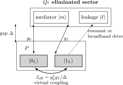
The same off-block coupling has two consequences. A virtual round trip through a well-detuned mediator produces an effective logical interaction $J_{\mathrm{eff}}$, while real population transferred into $Q$ is leakage. Scale separation, pulse bandwidth, and evolution time determine which interpretation is controlled.

Two-Level Approximations

A qubit is a chosen two-dimensional information carrier, not necessarily an intrinsically two-level object. After eliminating other states, any Hermitian qubit Hamiltonian can be written

$$H_{\mathrm{q}} = c_0 I + \frac{\hbar}{2} \boldsymbol\omega\cdot\boldsymbol\sigma.$$

The scalar $c_0$ is irrelevant to an isolated qubit but can matter when comparing phases between different particle-number, ancilla, or code sectors. The vector $\boldsymbol\omega$ depends on the physical control parameters and on the frame in which the Hamiltonian is written.

A useful two-level model requires all of the following:

1. The retained pair remains separated from omitted levels throughout the protocol.
2. Static and driven matrix elements connecting $P$ and $Q$ are small compared with the relevant detunings.
3. The pulse spectrum does not overlap an omitted transition.
4. Dressed logical states and control operators are used consistently.
5. Leakage and phase errors stay small over the full gate time.

There is no device-wide statement that a system “is a qubit.” The same device can be accurately two-level for a weak, narrow-band pulse and strongly multilevel for a short or high-amplitude pulse.

Weakly anharmonic qubit

Consider the lowest three levels of a weakly anharmonic oscillator. Let

$$\alpha = \omega_{12}-\omega_{01}$$

be the anharmonicity in angular-frequency units. For a transmon-like spectrum, $\alpha$ is typically negative. Drive the $0\leftrightarrow1$ transition resonantly, transform to the rotating frame, and make the rotating-wave approximation. With a complex Rabi envelope $\Omega$, the Hamiltonian is

$$\frac{H_R}{\hbar} = \begin{pmatrix} 0 & \Omega^*/2 & 0\\ \Omega/2 & 0 & \sqrt{2}\,\Omega^*/2\\ 0 & \sqrt{2}\,\Omega/2 & \alpha \end{pmatrix}$$

in the basis

$$\left\{ \lvert0\rangle, \lvert1\rangle, \lvert2\rangle \right\}.$$

The $\sqrt2$ factor is the oscillator matrix-element ratio. If

$$\frac{\lvert\Omega\rvert}{\lvert\alpha\rvert} \ll 1,$$

then $\lvert2\rangle$ can be eliminated perturbatively. For an instantaneous logical amplitude $c_1$, the eliminated amplitude is approximately

$$c_2 \simeq - \frac{\Omega}{\sqrt2\,\alpha} c_1,$$

and the logical state $\lvert1\rangle$ acquires the shift

$$\frac{\delta H_{11}}{\hbar} \simeq - \frac{\lvert\Omega\rvert^2}{2\alpha}.$$

Thus leakage amplitude is first order in $\Omega/\alpha$, leakage probability is second order, and the coherent ac Stark shift is also second order. Retaining the shift while claiming exactly zero leakage is inconsistent unless the statement is explicitly about an ideal effective model.

For a time-dependent pulse, this instantaneous elimination is only the leading term. Rapid envelope variation introduces derivative corrections, and a short pulse has spectral weight near the $1\leftrightarrow2$ transition. Derivative-removal-by-adiabatic-gate control, usually called DRAG, adds a quadrature related to the envelope derivative to cancel leading leakage and phase error. The detailed pulse-design problem belongs to Optimal Control.

Leakage Makes Projected Evolution Nonunitary

Let

$$U(t) = e^{-iHt/\hbar}$$

be the exact physical propagator and define its computational block

$$M(t) = P U(t) P \big\vert_{\mathcal H_{\mathrm{comp}}}.$$

Even though $U(t)$ is unitary on the full physical space, $M(t)$ need not be unitary. For a normalized logical input $\lvert\psi\rangle$,

$$\begin{aligned} L_\psi(t) &= 1- \lVert M(t)\lvert\psi\rangle\rVert^2 \\ &= \lVert Q U(t)P\lvert\psi\rangle\rVert^2 \end{aligned}$$

is the probability that population has left the computational subspace.

For a $d$-dimensional computational space, two useful summaries are

$$L_{\mathrm{av}} = 1- \frac{1}{d} \operatorname{Tr} \left( M^\dagger M \right)$$

and

$$L_{\mathrm{wc}} = 1- \lambda_{\min} \left( M^\dagger M \right).$$

The first is the input-state average leakage, while the second is the largest leakage over normalized logical inputs.

If $M$ has full rank, its polar decomposition is

$$M = V R, \qquad R = \left( M^\dagger M \right)^{1/2},$$

where $V$ is unitary on the computational space and $R$ is positive. The factor $V$ isolates the coherent logical action; $R$ records state-dependent contraction due to leakage. If $M$ is singular, the corresponding polar factor is a partial isometry and is not unique on the lost subspace.

This distinction is operationally important:

• a Hermitian effective Hamiltonian can reproduce the coherent unitary $V$;
• it cannot by itself reproduce the contraction $R$;
• a leakage-aware model must therefore retain an error estimate, add explicit leakage states, or use an effective open-system description.

When leakage is treated as a channel or a trace-decreasing retained operation, its canonical home is Erasure and Loss Channels.

Perturbative Couplings

The most useful logical interactions are often absent at first order. They arise because two retained states couple to a common eliminated mediator.

Dispersive qubit–resonator coupling

For an ideal two-level qubit coupled to one resonator mode, the Jaynes–Cummings Hamiltonian is

$$\begin{aligned} H ={}& \hbar\omega_r a^\dagger a + \frac{\hbar\omega_q}{2}\sigma_z \\ &+ \hbar g \left( a\sigma_+ + a^\dagger\sigma_- \right). \end{aligned}$$

Define the detuning

$$\Delta = \omega_q-\omega_r.$$

In the dispersive regime,

$$\frac{g\sqrt{n+1}}{\lvert\Delta\rvert} \ll1$$

for every appreciably populated photon number $n$. Choose the anti-Hermitian generator

$$S = \frac{g}{\Delta} \left( a\sigma_+ - a^\dagger\sigma_- \right),$$

which satisfies

$$[S,H_0]=-V.$$

Expanding the transformed Hamiltonian gives

$$e^S H e^{-S} = H_0 + \frac{1}{2}[S,V] + O\!\left( \frac{g^3}{\Delta^2} \right).$$

With

$$\chi = \frac{g^2}{\Delta},$$

the result, up to an additive scalar, is

$$\begin{aligned} H_{\mathrm{disp}} ={}& \hbar\omega_r a^\dagger a + \frac{\hbar\omega_q}{2}\sigma_z \\ &+ \hbar\chi \left( a^\dagger a+\frac{1}{2} \right) \sigma_z. \end{aligned}$$

The resonator frequency therefore depends on the qubit state, and the qubit frequency depends on photon number. The same virtual admixture that produces this useful frequency pull also opens the resonator-mediated Purcell decay channel when the resonator is lossy. Real weakly anharmonic qubits modify $\chi$ through higher levels, so the ideal two-level expression is a scaling law rather than a precision calibration formula.

Two qubits coupled through a bus

Now couple two qubits to the same mode:

$$V = \hbar \sum_{i=1}^{2} g_i \left( a\sigma_i^+ + a^\dagger\sigma_i^- \right),$$

with detunings

$$\Delta_i = \omega_i-\omega_r.$$

Eliminating virtual bus excitations generates, among the individual dispersive shifts, the exchange interaction

$$H_{\mathrm{ex}} = \hbar J \left( \sigma_1^+\sigma_2^- + \sigma_1^-\sigma_2^+ \right),$$

where

$$J = \frac{g_1g_2}{2} \left( \frac{1}{\Delta_1} + \frac{1}{\Delta_2} \right).$$

This formula assumes the same rotating-wave and dispersive conventions as the starting Hamiltonian. In the zero-photon sector, a qubit excitation can visit the bus virtually and return on the other qubit. The bus remains only weakly populated, but it mediates a real logical interaction.

If the dressed qubit frequencies are brought into resonance, then

$$H_{\mathrm{ex}} = \frac{\hbar J}{2} \left( X_1X_2+Y_1Y_2 \right).$$

In the one-excitation basis

$$\left\{ \lvert10\rangle, \lvert01\rangle \right\},$$

this is simply $\hbar J\sigma_x$. A duration

$$t_{\mathrm{iSWAP}} = \frac{\pi}{2\lvert J\rvert}$$

produces an iSWAP-family operation, up to the sign convention for $J$ and removable one-qubit phases. Half that duration produces a square-root-of-iSWAP-family entangler.

If the dressed qubits are far detuned from one another, exchange averages away rather than producing a clean swap. If the bus or a higher qubit level becomes resonant, it must be restored to the retained space. These are changes of model space, not small calibration corrections.

From Effective Couplings to Effective Gates

After projection and frame changes, a general two-qubit logical Hamiltonian can be expanded as

$$\begin{aligned} H_{\mathrm{log}} ={}& cI + \frac{\hbar}{2} \sum_{j=1}^{2} \boldsymbol\omega_j\cdot\boldsymbol\sigma_j \\ &+ \frac{\hbar}{4} \sum_{\mu,\nu\in\{x,y,z\}} J_{\mu\nu} \sigma_\mu\otimes\sigma_\nu. \end{aligned}$$

The local terms determine single-qubit phases and rotations. The nonlocal coefficients determine the entangling content. Two common representatives are

$$H_{XY} = \frac{\hbar J}{2} \left( X_1X_2+Y_1Y_2 \right)$$

and

$$H_{ZZ} = \frac{\hbar\zeta}{4} Z_1Z_2.$$

Evolution under $H_{ZZ}$ for

$$\zeta t=\pi$$

is locally equivalent to a controlled-$Z$ gate. “Locally equivalent” matters: single-qubit $Z$ phases and frame updates must be included before comparing the physical propagator with a named circuit gate. The Quantum Gates reference supplies standard matrix conventions.

Gate validation in the full model

Deriving a coefficient such as $J$ or $\zeta$ is not yet a gate validation. A useful comparison starts from the full propagator at the proposed gate time:

1. Form $M=PUP$ on the computational space.
2. Compute average and worst-case leakage from $M^\dagger M$.
3. Extract the coherent polar factor $V$.
4. Remove the declared rotating-frame and local phase conventions.
5. Compare $V$ with the target gate $G$.

For unitary $V$ and $G$ acting on a $d$-dimensional logical space, the average gate fidelity is

$$F_{\mathrm{avg}}(V,G) = \frac{ \left| \operatorname{Tr} \left( G^\dagger V \right) \right|^2+d }{ d(d+1) }.$$

This fidelity measures coherent mismatch after leakage has been separated. Reporting it without a leakage metric can hide a substantial failure of the logical subspace.

For an open physical system, $U$ must be replaced by a quantum channel or process map. A non-Hermitian Hamiltonian inserted by hand generally does not provide a trace-preserving gate model. Dissipative elimination must transform both coherent and jump terms, as developed in Adiabatic Elimination.

Perturbative Gadgets Preview

A perturbative gadget uses strongly penalized auxiliary degrees of freedom to generate a desired low-energy interaction that is absent microscopically. The method is conceptually the same virtual-process construction used for dispersive gates, but its purpose is Hamiltonian simulation or complexity reduction rather than hardware simplification.

As a minimal example, let an ancilla have penalty Hamiltonian

$$H_0 = \Delta \lvert1\rangle_a\langle1\rvert, \qquad \Delta\gt0,$$

and retain the ancilla ground state

$$P = I_{\mathrm{sys}} \otimes \lvert0\rangle_a\langle0\rvert.$$

Couple it to two Hermitian system operators $A$ and $B$ through

$$V = \lambda (A+B) \otimes X_a.$$

Because $PVP=0$, the leading logical effect is second order:

$$\begin{aligned} H_{\mathrm{eff}}^{(2)} &= - P V Q \frac{1}{\Delta} Q V P \\ &= - \frac{\lambda^2}{\Delta} (A+B)^2 \otimes \lvert0\rangle_a\langle0\rvert. \end{aligned}$$

If $A$ and $B$ act on different subsystems and satisfy

$$A^2=B^2=I, \qquad [A,B]=0,$$

then

$$(A+B)^2 = 2I+2AB.$$

Dropping the additive scalar leaves the induced interaction

$$H_{\mathrm{target}} = - \frac{2\lambda^2}{\Delta} AB.$$

The ancilla is only virtually excited, with amplitude of order $\lambda/\Delta$. The useful target scale is of order $\lambda^2/\Delta$, while higher-order errors are suppressed by additional powers of $\lambda/\Delta$.

This simple algebra does not make a gadget automatically practical. A credible construction must track:

• the norm of every coupling relative to the penalty gap;
• competing lower-order terms and required counterterms;
• the many-body gap after all gadgets are combined;
• ancilla preparation and leakage out of the penalty sector;
• how the target energy scale shrinks as the approximation improves;
• the number, locality, and precision of auxiliary couplings.

Perturbative gadgets are therefore controlled low-energy simulations, not free replacements of difficult interactions by easy ones. Their complexity-theoretic constructions belong in the future quantum-information volume.

Practical Validity Checklist

Before using an effective Hamiltonian as a gate model, record:

Question	Diagnostic
What is the computational space?	Give $P$, the encoding, and the basis ordering.
What is eliminated?	List leakage levels, buses, couplers, modes, and high-energy states in $Q$.
What is the scale hierarchy?	Compare coupling, detuning, anharmonicity, drive amplitude, bandwidth, and inverse gate time.
Which frame is used?	State every exact rotating or interaction-picture transformation.
What order is retained?	Name the expansion parameter and the first omitted order.
Are states and controls dressed?	Transform preparation, measurement, and drive operators consistently.
Is evolution actually unitary in $P$?	Evaluate $M^\dagger M$ and report leakage separately.
Does the intended gate appear?	Compare the full-model propagator with the target after local phases and frames are removed.
Are losses relevant?	Use an effective channel or master equation when dissipation competes with gate dynamics.
Has the model been benchmarked?	Compare spectra and time evolution with a larger truncation across the operating range.

An effective Hamiltonian is most useful when it turns these questions into explicit numbers. A compact logical matrix without such a record is a hypothesis, not yet a controlled model.

Common Mistakes

• Identifying a convenient pair of levels with an exact qubit without testing drive-induced leakage.
• Projecting to $PHP$ and omitting virtual energy shifts or mediated interactions.
• Using a dispersive coefficient outside the photon-number or detuning range in which it was derived.
• Calling the computational block $PUP$ unitary when population can leave the subspace.
• Comparing a rotating-frame effective propagator directly with a lab-frame gate matrix.
• Ignoring local phases when naming an entangling gate.
• Keeping a coherent effective Hamiltonian while discarding dissipation generated by the same eliminated mediator.
• Treating a perturbative gadget’s target term as exact while omitting its penalty and higher-order errors.

Cross-Links

• Effective Hamiltonians and Scale Separation
• Effective Hamiltonians in Quantum Matter
• Projection Methods
• Schrieffer–Wolff Transformation
• Adiabatic Elimination
• Rotating-Wave Approximation
• Average Hamiltonian Theory
• Two-Level Systems
• Quantum Information: Symmetry Application Map
• Circuit QED
• Erasure and Loss Channels
• Optimal Control
• Quantum Gates

References

1. S. Bravyi, D. P. DiVincenzo, and D. Loss, “Schrieffer–Wolff transformation for quantum many-body systems,” Annals of Physics 326, 2793–2826 (2011).
2. A. Blais, R.-S. Huang, A. Wallraff, S. M. Girvin, and R. J. Schoelkopf, “Cavity quantum electrodynamics for superconducting electrical circuits: An architecture for quantum computation,” Physical Review A 69, 062320 (2004).
3. J. Koch, T. M. Yu, J. Gambetta, A. A. Houck, D. I. Schuster, J. Majer, A. Blais, M. H. Devoret, S. M. Girvin, and R. J. Schoelkopf, “Charge-insensitive qubit design derived from the Cooper pair box,” Physical Review A 76, 042319 (2007).
4. F. Motzoi, J. M. Gambetta, P. Rebentrost, and F. K. Wilhelm, “Simple pulses for elimination of leakage in weakly nonlinear qubits,” Physical Review Letters 103, 110501 (2009).
5. A. Blais, A. L. Grimsmo, S. M. Girvin, and A. Wallraff, “Circuit quantum electrodynamics,” Reviews of Modern Physics 93, 025005 (2021).
6. J. Kempe, A. Kitaev, and O. Regev, “The complexity of the local Hamiltonian problem,” SIAM Journal on Computing 35, 1070–1097 (2006).
7. S. P. Jordan and E. Farhi, “Perturbative gadgets at arbitrary orders,” Physical Review A 77, 062329 (2008).
8. M. A. Nielsen and I. L. Chuang, Quantum Computation and Quantum Information, 10th anniversary ed., Cambridge University Press (2010).

Exercises

Leakage from a weakly anharmonic qubit

For the three-level rotating-frame Hamiltonian above, assume $\Omega$ is constant and $\lvert\alpha\rvert\gg\lvert\Omega\rvert$. Eliminate $c_2$ from the Schrödinger equation and derive the leading correction to the logical Hamiltonian. What leakage probability scale follows for a state with $c_1=1$?

Solution

The equation for the eliminated amplitude is

$$i\dot c_2 = \frac{\Omega}{\sqrt2}c_1 + \alpha c_2.$$

At leading adiabatic order, set $\dot c_2\simeq0$:

$$c_2 \simeq - \frac{\Omega}{\sqrt2\,\alpha} c_1.$$

The equation for $c_1$ contains the contribution

$$\frac{\Omega^*}{\sqrt2}c_2 \simeq - \frac{\lvert\Omega\rvert^2}{2\alpha} c_1.$$

Therefore

$$\delta H_{\mathrm{log}} = - \frac{\hbar\lvert\Omega\rvert^2}{2\alpha} \lvert1\rangle\langle1\rvert.$$

For $c_1=1$, the leading eliminated-state population is

$$\lvert c_2\rvert^2 \simeq \frac{\lvert\Omega\rvert^2}{2\lvert\alpha\rvert^2}.$$

This is an instantaneous perturbative estimate. Pulse edges and spectral overlap can produce additional leakage.

Projected evolution and leakage

Prove that

$$I_{\mathrm{comp}}-M^\dagger M$$

is positive semidefinite when $M=PUP$ is the computational block of a unitary $U$.

Solution

Define the positive-semidefinite candidate

$$D = I_{\mathrm{comp}}-M^\dagger M.$$

For any normalized $\lvert\psi\rangle$ in the computational subspace,

$$\begin{aligned} \langle\psi\lvert D\rvert\psi\rangle &= 1- \lVert PUP\lvert\psi\rangle\rVert^2 \\ &= \lVert QUP\lvert\psi\rangle\rVert^2 \ge0. \end{aligned}$$

The second equality follows from $P+Q=I$, $PQ=0$, and norm preservation by $U$. Since the quadratic form is nonnegative for every logical input, the operator is positive semidefinite.

Dispersive commutator

Using

$$S = \frac{g}{\Delta} \left( a\sigma_+-a^\dagger\sigma_- \right),$$

show that the second-order term $\frac12[S,V]$ produces the dispersive shift.

Solution

Let

$$A=a\sigma_+, \qquad B=a^\dagger\sigma_-.$$

Then

$$[A,B] = \frac{1}{2} \left[ 1+ \left( 2a^\dagger a+1 \right)\sigma_z \right].$$

Because

$$[A-B,A+B]=2[A,B],$$

one obtains

$$\frac{1}{2}[S,V] = \frac{\hbar g^2}{2\Delta} \left[ 1+ \left( 2a^\dagger a+1 \right)\sigma_z \right].$$

The first term is an additive scalar. With $\chi=g^2/\Delta$, the remaining term is

$$\hbar\chi \left( a^\dagger a+\frac12 \right)\sigma_z,$$

which is the stated dispersive interaction.

Bus-mediated exchange gate

Two identical qubits have equal dispersive couplings $g$ and detunings $\Delta$ from a common bus. Find $J$ and the duration of a square-root-of-iSWAP-family gate after the dressed qubits are tuned into mutual resonance.

Solution

The exchange coefficient is

$$J = \frac{g^2}{2} \left( \frac{1}{\Delta} + \frac{1}{\Delta} \right) = \frac{g^2}{\Delta}.$$

In the one-excitation subspace,

$$H_{\mathrm{ex}} = \hbar J\sigma_x.$$

A full iSWAP-family transfer requires $\lvert J\rvert t=\pi/2$. Its square root therefore requires

$$t_{\sqrt{\mathrm{iSWAP}}} = \frac{\pi}{4\lvert J\rvert} = \frac{\pi\lvert\Delta\rvert}{4g^2}.$$

The result assumes the dispersive condition $g/\lvert\Delta\rvert\ll1$, negligible loss, a vacuum bus, and compensated one-qubit phases.

Coherent error versus leakage

Suppose a two-dimensional computational block has polar decomposition

$$M = V \begin{pmatrix} 1&0\\ 0&\sqrt{1-\epsilon} \end{pmatrix}, \qquad 0\le\epsilon\le1.$$

Find $L_{\mathrm{av}}$ and $L_{\mathrm{wc}}$. Can the unitary $V$ alone reveal the leakage?

Solution

Here

$$M^\dagger M = \begin{pmatrix} 1&0\\ 0&1-\epsilon \end{pmatrix}.$$

Therefore

$$L_{\mathrm{av}} = 1- \frac{2-\epsilon}{2} = \frac{\epsilon}{2},$$

while

$$L_{\mathrm{wc}} = 1-(1-\epsilon) = \epsilon.$$

The polar unitary $V$ contains only the coherent logical action. It does not reveal the contraction and therefore cannot by itself reveal either leakage measure.

Second-order perturbative gadget

For the ancilla gadget above, take $A=Z_1$ and $B=Z_2$. Derive the nonconstant effective interaction and estimate the eliminated-ancilla population scale.

Solution

Since $Z_1$ and $Z_2$ commute and square to the identity,

$$\left( Z_1+Z_2 \right)^2 = 2I+2Z_1Z_2.$$

The second-order Hamiltonian is

$$H_{\mathrm{eff}}^{(2)} = - \frac{2\lambda^2}{\Delta} \left( I+Z_1Z_2 \right).$$

After dropping the scalar term, the induced interaction is

$$H_{\mathrm{target}} = - \frac{2\lambda^2}{\Delta} Z_1Z_2.$$

The excited-ancilla amplitude is of order $\lambda/\Delta$ times an eigenvalue scale of $Z_1+Z_2$, so its population is of order $(\lambda/\Delta)^2$, with a state-dependent factor bounded by the squared operator norm.