Tight-Binding Models

A tight-binding model represents crystalline quantum states in a retained set of localized orbitals and replaces continuum motion by coherent Hamiltonian matrix elements between them. Translation symmetry then converts the real-space hopping matrices into a finite-dimensional Bloch Hamiltonian $h(\mathbf k)$ for each crystal momentum.

The method is not synonymous with nearest-neighbor hopping, one orbital per site, or nonoverlapping atomic orbitals. A tight-binding representation can contain many orbitals, long-range and complex hopping, spin–orbit coupling, nonorthogonal basis functions, and parameters downfolded from first-principles bands. Its accuracy is controlled by the chosen subspace and the terms retained after projection.

This page is the canonical home for tight binding as a quantum-matter modeling method: localized-basis construction, crystalline hopping matrices, orbital embedding, multi-orbital Bloch Hamiltonians, spin-dependent terms, material-band validation, and the Wannier and Hubbard bridges. Tight-Binding Model owns the generic graph Hamiltonian, Fock-space occupation, finite boundaries, and detailed chain solution.

Flat Bands owns the special momentum-independent case, including compact localized states, singular touchings, spectral flattening, projector geometry, and flat-band ferromagnetism.

Required background. Bloch’s Theorem supplies the translation-sector decomposition, while Crystals and Lattices supplies primitive cells, motifs, orbital positions, and finite geometry.

Localized Orbital Basis

Choose localized one-particle states

$$|\mathbf R,\alpha\rangle,$$

where $\mathbf R$ labels a Bravais-lattice cell and $\alpha=1,\ldots,N_{\mathrm{orb}}$ labels an orbital, sublattice, layer, or other retained mode within the cell. Translation covariance means

$$|\mathbf R,\alpha\rangle = T_{\mathbf R} |\mathbf0,\alpha\rangle.$$

For an orthonormal basis,

$$\langle \mathbf R,\alpha | \mathbf R',\beta \rangle = \delta_{\mathbf R\mathbf R'} \delta_{\alpha\beta}.$$

The corresponding real-space wavefunctions are

$$w_{\mathbf R\alpha}(\mathbf r) = \langle\mathbf r|\mathbf R,\alpha\rangle.$$

They may be idealized atomic orbitals, symmetry-adapted combinations, molecular orbitals, numerically constructed Wannier functions, or phenomenological modes. The word “orbital” describes a basis state, not necessarily an isolated-atom eigenfunction.

Projection from a continuum Hamiltonian

Given a one-particle operator $\widehat h$, its projected matrix elements are

$$t_{\alpha\beta}(\boldsymbol\Delta) \equiv \langle \mathbf0,\alpha | \widehat h | \boldsymbol\Delta,\beta \rangle.$$

Translation symmetry makes the matrix element depend only on the cell displacement:

$$\langle \mathbf R,\alpha | \widehat h | \mathbf R+\boldsymbol\Delta,\beta \rangle = t_{\alpha\beta}(\boldsymbol\Delta).$$

If the retained orbitals span an invariant subspace and every matrix element is kept, this is an exact change of representation within that subspace. Approximation enters when remote states are excluded, energy dependence from downfolding is neglected, or long-range matrix elements are truncated.

Basis nonuniqueness

Localized orbitals are not observables. A unitary transformation among retained orbitals changes individual onsite energies, hopping amplitudes, and spatial spreads while preserving predictions when all operators are transformed consistently. Statements such as “the nearest-neighbor hopping is $t$” are meaningful only after the basis, gauge, orbital embedding, and fitting procedure are specified.

Real-Space Hamiltonian

Using the hopping orientation fixed in Conventions for Quantum Matter, write

$$H_0 = \sum_{\mathbf R,\boldsymbol\Delta} \sum_{\alpha,\beta} t_{\alpha\beta}(\boldsymbol\Delta) c_{\mathbf R\alpha}^{\dagger} c_{\mathbf R+\boldsymbol\Delta,\beta}.$$

$t_{\alpha\beta}(\boldsymbol\Delta)$ multiplies the transfer from orbital $(\mathbf R+\boldsymbol\Delta,\beta)$ to $(\mathbf R,\alpha)$. Hermiticity requires

$$t_{\alpha\beta}(\boldsymbol\Delta) = t_{\beta\alpha}^{\ast}(-\boldsymbol\Delta).$$

The $\boldsymbol\Delta=\mathbf0$ block contains onsite energies and intracell hybridization. In a basis that diagonalizes that block,

$$t_{\alpha\beta}(\mathbf0) = \epsilon_{\alpha}\delta_{\alpha\beta},$$

but diagonal onsite form is a convenience rather than a requirement.

Hopping is coherent

A hopping amplitude is an off-diagonal Hamiltonian matrix element. It produces unitary superposition and interference; it is not a classical rate or a stochastic jump probability. The probability of transfer depends on the full time evolution, all available paths, detuning, and state preparation.

The conventional minus sign

For one orbital on a chain, it is common to write

$$H = \epsilon_0\sum_j c_j^{\dagger}c_j - t\sum_j \left( c_j^{\dagger}c_{j+1} + c_{j+1}^{\dagger}c_j \right),$$

with $t>0$. In the general convention above,

$$t(+a) = t(-a) = -t.$$

Some sources instead call the signed matrix element itself $t$. Always infer the sign from the written Hamiltonian before comparing dispersions.

Bloch Hamiltonian

Use the cell-convention transform

$$\begin{aligned} c_{\mathbf k\alpha} &= \frac{1}{\sqrt{N_c}} \sum_{\mathbf R} e^{-i\mathbf k\cdot\mathbf R} c_{\mathbf R\alpha}, \\ c_{\mathbf R\alpha} &= \frac{1}{\sqrt{N_c}} \sum_{\mathbf k} e^{i\mathbf k\cdot\mathbf R} c_{\mathbf k\alpha}. \end{aligned}$$

Substitution gives

$$H_0 = \sum_{\mathbf k} \mathbf c_{\mathbf k}^{\dagger} h(\mathbf k) \mathbf c_{\mathbf k},$$

with

$$h_{\alpha\beta}(\mathbf k) = \sum_{\boldsymbol\Delta} t_{\alpha\beta}(\boldsymbol\Delta) e^{i\mathbf k\cdot\boldsymbol\Delta}.$$

Hermiticity in real space implies

$$h^{\dagger}(\mathbf k) = h(\mathbf k).$$

The cell convention also makes the matrix periodic:

$$h(\mathbf k+\mathbf G) = h(\mathbf k).$$

At each $\mathbf k$, solve

$$h(\mathbf k) u_n(\mathbf k) = \varepsilon_n(\mathbf k) u_n(\mathbf k).$$

With $N_{\mathrm{orb}}$ orthonormal spinless orbitals per primitive cell, there are $N_{\mathrm{orb}}$ bands and $N_cN_{\mathrm{orb}}$ one-particle states in a finite periodic crystal. Physical spin doubles this count before spin splitting or additional constraints are considered.

Band operators

Choose normalized eigenvectors,

$$u_m^{\dagger}(\mathbf k) u_n(\mathbf k) = \delta_{mn},$$

and define

$$\gamma_{n\mathbf k} = \sum_{\alpha} u_{n\alpha}^{\ast}(\mathbf k) c_{\mathbf k\alpha}.$$

Then

$$H_0 = \sum_{n,\mathbf k} \varepsilon_n(\mathbf k) \gamma_{n\mathbf k}^{\dagger} \gamma_{n\mathbf k}.$$

The diagonalization is exact for the specified quadratic model. Whether that model accurately represents a material is a separate question.

Orbital Embedding and Bloch Gauge

The cell transform excludes the basis position $\boldsymbol\tau_\alpha$. An orbital-position convention instead uses

$$\bar c_{\mathbf k\alpha} = \frac{1}{\sqrt{N_c}} \sum_{\mathbf R} e^{-i\mathbf k\cdot (\mathbf R+\boldsymbol\tau_\alpha)} c_{\mathbf R\alpha}.$$

Define

$$D_{\alpha\beta}(\mathbf k) = \delta_{\alpha\beta} e^{-i\mathbf k\cdot\boldsymbol\tau_\alpha}.$$

Then

$$\bar{\mathbf c}_{\mathbf k} = D(\mathbf k)\mathbf c_{\mathbf k},$$

and

$$\bar h(\mathbf k) = D(\mathbf k) h(\mathbf k) D^{\dagger}(\mathbf k).$$

The eigenvalues are identical, but the embedded matrix is generally sewn rather than strictly periodic:

$$\bar h(\mathbf k+\mathbf G) = D_{\mathbf G} \bar h(\mathbf k) D_{\mathbf G}^{\dagger}.$$

Orbital embedding matters for position, polarization, optical matrix elements, and Berry geometry. Two Hamiltonian matrices that look different can represent the same model in different $\mathbf k$-dependent bases.

Nonorthogonal Orbitals

Atomic-orbital bases often have a nontrivial overlap,

$$S_{\alpha\beta}(\boldsymbol\Delta) = \langle \mathbf0,\alpha | \boldsymbol\Delta,\beta \rangle.$$

Its Bloch transform is

$$S_{\alpha\beta}(\mathbf k) = \sum_{\boldsymbol\Delta} S_{\alpha\beta}(\boldsymbol\Delta) e^{i\mathbf k\cdot\boldsymbol\Delta}.$$

The band problem is then generalized:

$$h(\mathbf k)u_n(\mathbf k) = \varepsilon_n(\mathbf k) S(\mathbf k)u_n(\mathbf k).$$

For a linearly independent basis, $S(\mathbf k)$ must be positive definite. Replacing this by an ordinary eigenproblem without first orthogonalizing the basis changes the spectrum. Orthogonalization itself can lengthen the range of the effective hopping, so “nearest neighbor” is not basis invariant.

Hopping Range and Locality

For well-localized orbitals and a local or short-ranged one-particle operator, matrix elements often decay with the separation

$$|\boldsymbol\Delta + \boldsymbol\tau_\beta - \boldsymbol\tau_\alpha|.$$

This motivates truncation to onsite, nearest-neighbor, or a few neighbor shells. The decay can be anisotropic and orbital dependent, and downfolding can generate longer-range terms even when the original microscopic Hamiltonian was local.

A hopping cutoff should be justified by a convergence test. Compare full and truncated models over the entire target Brillouin zone, not only along a few high-symmetry lines.

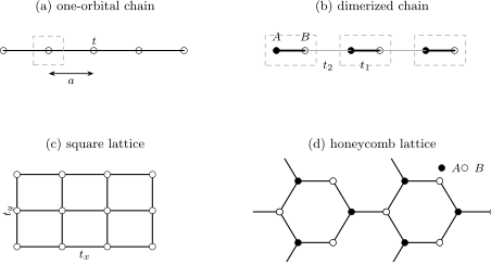
The same localized-orbital method produces different Bloch matrices once the Bravais lattice, motif, and retained hopping graph are specified. A one-orbital chain has one band; the dimerized and honeycomb examples have two orbitals per primitive cell and therefore two bands before spin.

Worked Example: One-Dimensional Chain

For the Hamiltonian written above,

$$h(k) = \epsilon_0 - t e^{ika} - t e^{-ika},$$

so

$$\varepsilon(k) = \epsilon_0 - 2t\cos(ka).$$

For $t>0$, the minimum is at $k=0$, the maximum is at $k=\pi/a$, and the bandwidth is

$$W = 4t.$$

The dispersion is broad when neighboring orbitals hybridize strongly and collapses to the atomic level $\epsilon_0$ as $t\to0$. The Tight-Binding Chain dossier develops boundaries, finite spectra, normalization, and validation tests in full.

Worked Example: SSH Chain

The Su–Schrieffer–Heeger chain has two orbitals $A,B$ per cell, intracell hopping $t_1$, and intercell hopping $t_2$. With real hoppings,

$$H = - \sum_R \left[ t_1 a_R^{\dagger}b_R + t_2 a_{R+a}^{\dagger}b_R + \mathrm{h.c.} \right].$$

In the cell convention,

$$h(k) = - \begin{pmatrix} 0 & t_1+t_2e^{-ika} \\ t_1+t_2e^{ika} & 0 \end{pmatrix}.$$

The bands are

$$\varepsilon_{\pm}(k) = \pm \sqrt{ t_1^2+t_2^2 + 2t_1t_2\cos(ka) }.$$

For positive $t_1,t_2$, the direct gap at $k=\pi/a$ is

$$E_{\mathrm g} = 2|t_1-t_2|.$$

The gap closes at $t_1=t_2$, where the chosen two-site cell merely folds the uniform chain. Boundary zero modes and the topological distinction require chiral symmetry, a declared termination, and careful unit-cell conventions; SSH Model is the canonical model dossier.

Worked Example: Square Lattice

For one orbital per rectangular cell and nearest-neighbor hoppings $t_x,t_y$,

$$\varepsilon(\mathbf k) = \epsilon_0 - 2t_x\cos(k_xa_x) - 2t_y\cos(k_ya_y).$$

If $t_x,t_y>0$, the bandwidth is

$$W = 4(t_x+t_y).$$

For the isotropic square lattice,

$$t_x=t_y=t,$$

the band runs from $\epsilon_0-4t$ at $\Gamma$ to $\epsilon_0+4t$ at the zone corner. The saddle points at $(\pi/a,0)$ and $(0,\pi/a)$ later produce a two-dimensional van Hove singularity in the density of states.

Longer-range diagonal hopping $t'$ adds

$$-4t' \cos(k_xa) \cos(k_ya),$$

changing particle–hole symmetry and the Fermi-surface shape without changing the one-orbital band count.

Worked Example: Honeycomb Lattice

The honeycomb structure is not a Bravais lattice. It has a triangular Bravais lattice and two sublattices $A,B$. For nearest-neighbor hopping in a common cell convention,

$$h(\mathbf k) = -t \begin{pmatrix} 0 & f(\mathbf k) \\ f^{\ast}(\mathbf k) & 0 \end{pmatrix},$$

where one convenient choice is

$$f(\mathbf k) = 1 + e^{-i\mathbf k\cdot\mathbf a_1} + e^{-i\mathbf k\cdot\mathbf a_2}.$$

The bands are

$$\varepsilon_{\pm}(\mathbf k) = \pm t|f(\mathbf k)|.$$

They touch where

$$f(\mathbf K) = 0,$$

at inequivalent Brillouin-zone corners. Expanding near such a point gives a two-component Dirac Hamiltonian whose Pauli matrices act on sublattice pseudospin, not physical spin.

An onsite sublattice imbalance adds

$$h_{\Delta} = \Delta\sigma_z$$

and opens a gap $2|\Delta|$ in this minimal model. Graphene Dirac Model owns the compact low-energy convention. Graphene and Dirac Materials develops the material interpretation, pseudospin and Berry diagnostics, magnetic spectrum, realistic corrections, and moiré bridge.

Multi-Orbital Models

With several orbitals per cell, $h(\mathbf k)$ is an $N_{\mathrm{orb}}\times N_{\mathrm{orb}}$ Hermitian matrix. Its entries can include:

• crystal-field-split onsite energies;
• intracell hybridization between orbitals of compatible symmetry;
• direction-dependent intercell hopping;
• longer-range hopping;
• layer and sublattice couplings;
• spin-dependent onsite and hopping terms.

Orbital symmetry strongly constrains the angular dependence. Slater–Koster parameterizations organize two-center matrix elements such as $ss\sigma$, $sp\sigma$, $pp\sigma$, and $pp\pi$ by bond direction. Their tabulated form is a modeling convention, not a substitute for checking the retained basis and environment.

Symmetry covariance

If a crystal symmetry $g$ maps $\mathbf k$ to $g\mathbf k$, a correctly constructed Bloch Hamiltonian obeys

$$U_g(\mathbf k) h(\mathbf k) U_g^{\dagger}(\mathbf k) = h(g\mathbf k),$$

with possible reciprocal sewing when $g\mathbf k$ is returned to the chosen zone. Symmetry can force degeneracies, forbid hybridization, or relate hopping parameters, but it does not determine their numerical values.

Symmetry of Bloch States owns the representation-theoretic interpretation of $U_g(\mathbf k)$, little-group labels, compatibility relations, and protected versus avoided crossings. This page owns constructing the hopping model and verifying its covariance under the declared symmetries.

Spin–Orbit Coupling

With physical spin, each orbital carries a spinor and $h(\mathbf k)$ acts in orbital $\otimes$ spin space. Atomic spin–orbit coupling takes the onsite form

$$H_{\mathrm{SOC}}^{\mathrm{atom}} = \lambda \sum_{\mathbf R} \mathbf L_{\mathbf R} \cdot \mathbf S_{\mathbf R}.$$

It requires an orbital basis on which $\mathbf L$ is represented; inserting $\lambda\mathbf L\cdot\mathbf S$ into a one-orbital scalar model is generally meaningless.

A generic spin-dependent hopping block can be written

$$t(\boldsymbol\Delta) = t_0(\boldsymbol\Delta)I_2 + i\boldsymbol\lambda(\boldsymbol\Delta) \cdot \boldsymbol\sigma.$$

For real coefficients and time-reversal-compatible hopping,

$$t_0(-\boldsymbol\Delta) = t_0(\boldsymbol\Delta),$$ $$\boldsymbol\lambda(-\boldsymbol\Delta) = -\boldsymbol\lambda(\boldsymbol\Delta).$$

The odd spin-dependent term becomes momentum odd. The full spinful Bloch matrix must satisfy the appropriate time-reversal, point-group, and Hermiticity constraints. Spin–Orbit Coupling owns the angular-momentum operator. Spin–Orbit Coupling in Solids develops crystal-field projection, Bloch-band symmetry constraints, and Rashba and Dresselhaus invariants; a material model must still specify its orbital and spatial symmetry representation.

Complex Hopping and Magnetic Phases

Local orbital rephasings,

$$c_i \longrightarrow e^{i\chi_i}c_i,$$

move phases among bonds without changing gauge-invariant loop products. A magnetic vector potential can be incorporated approximately through the Peierls phase,

$$t_{ij} \longrightarrow t_{ij} \exp \left[ \frac{iq}{\hbar} \int_{\mathbf r_j}^{\mathbf r_i} \mathbf A\cdot d\boldsymbol\ell \right].$$

Only the accumulated phase around a closed loop is directly tied to magnetic flux. The path choice, orbital extent, and additional magnetic couplings must be controlled in precision work; see Peierls Phase Preview.

From Bands to Wannier Functions

Wannier Functions is the canonical home for the exact Bloch-subspace-to-localized-basis theory, including gauge, localization, and obstruction conditions. Wannierization Workflows owns numerical windows, trials, disentanglement, spread and mesh convergence, and the validated real-space matrix artifacts. This page resumes once that localized basis and hopping data are declared and owns the resulting crystalline tight-binding model and its validation.

For a complete localized basis, the band-derived hopping matrix is the inverse Fourier transform of the Wannier-gauge Bloch matrix:

$$t_{mn}(\boldsymbol\Delta) = \frac{1}{N_c} \sum_{\mathbf k} e^{-i\mathbf k\cdot\boldsymbol\Delta} h_{mn}(\mathbf k).$$

Within a fixed selected subspace, a unitary Bloch-frame change and complete Fourier transform are exact basis changes: they preserve the projector and the represented spectrum. Subspace selection or disentanglement, hopping truncation, parameter fitting, and errors in the reference electronic structure are separate entries in the approximation error ledger.

Relation to Hubbard Models

The base tight-binding Hamiltonian is quadratic. A Hubbard model adds interactions in the same localized basis, for example

$$H_{\mathrm{Hub}} = H_0 + \sum_{\mathbf R,\alpha} U_{\alpha} n_{\mathbf R\alpha\uparrow} n_{\mathbf R\alpha\downarrow}.$$

More complete projections generate interorbital repulsion, Hund exchange, pair hopping, and nonlocal density interactions. Their values depend on orbital localization and on what screening has already been included.

Adding $U$ does not merely “correct the band energies.” It changes the many-body problem and can invalidate an independent-particle description. Hubbard Model owns the interacting Hamiltonian, limits, and many-body diagnostics. Hubbard Physics in Materials owns screened interaction tensors, filling audits, double counting, and validation of the resulting material model.

Model-Construction Workflow

1. Define the target. State the energy window, observables, filling range, and accuracy required.
2. Choose the primitive cell and orbitals. Record $\mathbf a_i$, $\boldsymbol\tau_\alpha$, orbital character, spin convention, and local axes.
3. Specify the basis source. Distinguish empirical atomic orbitals, fitted symmetry models, Wannier functions, and formal toy orbitals.
4. Construct symmetry-allowed terms. Enforce Hermiticity, translations, point-group symmetries, time reversal, and any declared symmetry breaking.
5. Fit or compute parameters. Document data, first-principles method, energy window, objective function, and uncertainties.
6. Control truncation. Examine real-space decay and compare successive hopping ranges.
7. Validate globally. Compare bands and eigenvector-sensitive observables over the full zone, not only a high-symmetry path.
8. Archive conventions. Preserve orbital order, embeddings, phases, units, parameter provenance, and code version.

Validity and Diagnostics

A mature tight-binding model should pass:

• Hermiticity: $t(\boldsymbol\Delta)=t^{\dagger}(-\boldsymbol\Delta)$;
• mode count: $N_cN_{\mathrm{orb}}$ states before spin or Nambu enlargement;
• spectral periodicity: correct reciprocal sewing in the chosen basis;
• symmetry covariance: all declared exact symmetries act correctly;
• atomic limit: intercell hopping removed gives the intended local levels;
• range convergence: observables stabilize as hopping shells are added;
• gauge consistency: basis transformations leave physical predictions unchanged;
• target fidelity: bands, orbital weights, matrix elements, and responses match the source within stated tolerances.

Matching eigenvalues alone is insufficient when the model will be used for optical transitions, Berry curvature, polarization, or interactions. Those quantities depend on eigenvectors, orbital positions, and projected operators.

Common Mistakes

Calling the basis unique

Onsite energies and hoppings depend on the orbital gauge and downfolding. Quote the construction, not only the numbers.

Dropping the orbital embedding

The cell and orbital-position conventions have identical spectra but different matrix representatives. Mixing their eigenvectors, derivatives, or position operators produces incorrect geometric and optical quantities.

Treating a nonorthogonal basis as orthonormal

If $S(\mathbf k)\ne I$, solve the generalized eigenproblem or document the orthogonalization.

Guessing the sign of a hopping

The symbol $t$ may denote a positive magnitude or a signed matrix element. Read the Hamiltonian.

Truncating by geometric distance alone

Orbital orientation and downfolding can make a farther hopping larger than a nearer symmetry-suppressed one. Converge by matrix magnitude and target observables.

Confusing pseudospin with physical spin

Pauli matrices can act on sublattice, orbital, layer, Nambu, or physical-spin spaces. Label the tensor factor explicitly.

Inferring topology from a band plot

Band energies alone do not determine Berry phases, topological indices, or protected boundary states. The eigenvectors, symmetry representation, filling, and boundary must be specified. Chern Numbers in Band Theory gives the occupied-projector and numerical checks for the two-dimensional integer invariant.

Adding interactions without revisiting the basis

Changing orbital localization redistributes hopping and interaction matrix elements. A value of $U/t$ is not basis independent.

Exercises

Exercise 1: derive the Bloch matrix

Starting from

$$H_0 = \sum_{\mathbf R,\boldsymbol\Delta} \sum_{\alpha,\beta} t_{\alpha\beta}(\boldsymbol\Delta) c_{\mathbf R\alpha}^{\dagger} c_{\mathbf R+\boldsymbol\Delta,\beta},$$

derive $h_{\alpha\beta}(\mathbf k)$ in the cell convention.

Solution

Insert

$$c_{\mathbf R\alpha} = \frac{1}{\sqrt{N_c}} \sum_{\mathbf k} e^{i\mathbf k\cdot\mathbf R} c_{\mathbf k\alpha}.$$

Then

$$\begin{aligned} c_{\mathbf R\alpha}^{\dagger} c_{\mathbf R+\boldsymbol\Delta,\beta} &= \frac{1}{N_c} \sum_{\mathbf k,\mathbf k'} e^{-i\mathbf k\cdot\mathbf R} e^{i\mathbf k'\cdot (\mathbf R+\boldsymbol\Delta)} c_{\mathbf k\alpha}^{\dagger} c_{\mathbf k'\beta}. \end{aligned}$$

The sum over $\mathbf R$ gives

$$\sum_{\mathbf R} e^{i(\mathbf k'-\mathbf k)\cdot\mathbf R} = N_c\delta_{\mathbf k\mathbf k'}.$$

Therefore

$$H_0 = \sum_{\mathbf k,\alpha,\beta} \left[ \sum_{\boldsymbol\Delta} t_{\alpha\beta}(\boldsymbol\Delta) e^{i\mathbf k\cdot\boldsymbol\Delta} \right] c_{\mathbf k\alpha}^{\dagger} c_{\mathbf k\beta},$$

so

$$h_{\alpha\beta}(\mathbf k) = \sum_{\boldsymbol\Delta} t_{\alpha\beta}(\boldsymbol\Delta) e^{i\mathbf k\cdot\boldsymbol\Delta}.$$

Exercise 2: prove Hermiticity in momentum space

Use

$$t_{\alpha\beta}(\boldsymbol\Delta) = t_{\beta\alpha}^{\ast}(-\boldsymbol\Delta)$$

to prove $h^{\dagger}(\mathbf k)=h(\mathbf k)$.

Solution

Take the conjugate transpose:

$$\begin{aligned} \left[ h^{\dagger}(\mathbf k) \right]_{\alpha\beta} &= h_{\beta\alpha}^{\ast}(\mathbf k) \\ &= \sum_{\boldsymbol\Delta} t_{\beta\alpha}^{\ast}(\boldsymbol\Delta) e^{-i\mathbf k\cdot\boldsymbol\Delta} \\ &= \sum_{\boldsymbol\Delta} t_{\alpha\beta}(-\boldsymbol\Delta) e^{-i\mathbf k\cdot\boldsymbol\Delta}. \end{aligned}$$

Relabel $\boldsymbol\Delta'=-\boldsymbol\Delta$:

$$\left[ h^{\dagger}(\mathbf k) \right]_{\alpha\beta} = \sum_{\boldsymbol\Delta'} t_{\alpha\beta}(\boldsymbol\Delta') e^{i\mathbf k\cdot\boldsymbol\Delta'} = h_{\alpha\beta}(\mathbf k).$$

Exercise 3: chain bandwidth and sign

For

$$\varepsilon(k) = \epsilon_0-2t\cos(ka),$$

find the band edges and bandwidth for both signs of $t$.

Solution

Since $\cos(ka)\in[-1,1]$, the energy set is

$$\epsilon_0-2|t| \leq \varepsilon(k) \leq \epsilon_0+2|t|.$$

Thus

$$W = 4|t|.$$

For $t>0$, the minimum is at $k=0$ and the maximum at $k=\pi/a$. For $t<0$, those momenta exchange roles. The energy set is unchanged under $t\to-t$ on this bipartite nearest-neighbor chain, but the momentum assignment changes.

Exercise 4: SSH gap

Diagonalize the SSH Bloch matrix and determine when the bulk gap closes.

Solution

The off-diagonal amplitude is

$$q(k) = t_1+t_2e^{-ika}.$$

For

$$h(k) = - \begin{pmatrix} 0&q(k) \\ q^{\ast}(k)&0 \end{pmatrix},$$

the characteristic equation is

$$\varepsilon^2 = |q(k)|^2.$$

Therefore

$$\varepsilon_{\pm}(k) = \pm \sqrt{ t_1^2+t_2^2+2t_1t_2\cos(ka) }.$$

For positive hoppings, the minimum band separation occurs at $k=\pi/a$:

$$E_{\mathrm g} = 2|t_1-t_2|.$$

It closes when $t_1=t_2$. More generally, a closing requires $|t_1|=|t_2|$ at a momentum whose phase cancels the relative hopping phase.

Exercise 5: square-lattice checks

For isotropic nearest-neighbor hopping on a square lattice,

$$\varepsilon(\mathbf k) = -2t \left[ \cos(k_xa)+\cos(k_ya) \right],$$

find the energies at $\Gamma$, $X=(\pi/a,0)$, and $M=(\pi/a,\pi/a)$. Identify the saddle point.

Solution

Direct substitution gives

$$\varepsilon(\Gamma) = -4t,$$ $$\varepsilon(X) = 0,$$ $$\varepsilon(M) = 4t.$$

Near $X$, write

$$k_x = \frac{\pi}{a}+q_x, \qquad k_y = q_y.$$

To quadratic order,

$$\varepsilon \approx -t a^2q_x^2 + t a^2q_y^2.$$

The curvatures have opposite signs, so $X$ is a saddle point.

Exercise 6: honeycomb mass term

For

$$h(\mathbf k) = \begin{pmatrix} \Delta & -tf(\mathbf k) \\ -tf^{\ast}(\mathbf k) & -\Delta \end{pmatrix},$$

find the bands and the gap at a point where $f(\mathbf K)=0$.

Solution

The characteristic equation is

$$\varepsilon^2 = \Delta^2 + t^2|f(\mathbf k)|^2.$$

Thus

$$\varepsilon_{\pm}(\mathbf k) = \pm \sqrt{ \Delta^2+t^2|f(\mathbf k)|^2 }.$$

At $\mathbf K$,

$$\varepsilon_{\pm}(\mathbf K) = \pm|\Delta|,$$

so the direct gap is $2|\Delta|$. The Pauli matrix associated with $\Delta$ acts on the $A/B$ sublattice space.

Exercise 7: generalized eigenproblem

Suppose a nonorthogonal two-orbital basis has positive-definite overlap matrix $S(\mathbf k)$. Show how to convert

$$h(\mathbf k)u = \varepsilon S(\mathbf k)u$$

into an ordinary Hermitian eigenproblem.

Solution

Positive definiteness gives a Hermitian square root $S^{1/2}$ and inverse $S^{-1/2}$. Set

$$v = S^{1/2}u.$$

Multiplying the generalized equation by $S^{-1/2}$ gives

$$\left[ S^{-1/2} h S^{-1/2} \right] v = \varepsilon v.$$

The transformed Hamiltonian is Hermitian because $h$ and $S^{-1/2}$ are Hermitian:

$$\left( S^{-1/2}hS^{-1/2} \right)^{\dagger} = S^{-1/2}hS^{-1/2}.$$

This symmetric orthogonalization preserves the generalized eigenvalues but changes the real-space shape and range of the effective orbitals and hopping.

Connections

• The chapter gateway helps choose this localized-orbital branch and routes its bands to state counting, Fermi-surface, topology, or interacting-model owners.
• Band Theory Overview connects model eigenvalues to filling, material behavior, Kohn–Sham bands, and interacting quasiparticle spectra.
• Bloch’s Theorem explains why translation reduces the problem to independent crystal-momentum sectors.
• Nearly Free Electrons is the complementary weak-potential, plane-wave expansion.
• Density of States turns the resulting band dispersions into normalized energy distributions and van Hove diagnostics.
• Fermi Surface turns partially filled tight-binding bands into material-facing sheets, pockets, and low-energy kinematics.
• Chern Numbers in Band Theory develops a regulated two-band model, symmetry constraints, and gauge-invariant Brillouin-zone computation.
• Tight-Binding Model owns arbitrary graphs, second quantization, boundary conditions, and many-particle occupation of quadratic modes.
• Tight-Binding Chain is the convention-complete one-dimensional dossier.
• SSH Model and Graphene Dirac Model are compact model references.
• Graphene and Dirac Materials follows the honeycomb model into experimentally diagnostic Dirac physics and moiré minibands.
• Graphene tracks how bond deformation, sublattice asymmetry, gauge fields, substrates, and twist alter that honeycomb baseline in engineered devices.
• Hubbard Model develops the interacting extension.
• Hubbard Physics in Materials follows the localized basis into screened interactions and material validation.
• Conventions for Quantum Matter fixes Fourier phases, hopping orientation, orbital embedding, and reciprocal sewing.

References

1. J. C. Slater and G. F. Koster, “Simplified LCAO Method for the Periodic Potential Problem,” Physical Review 94, 1498–1524 (1954), doi:10.1103/PhysRev.94.1498.
2. G. H. Wannier, “The Structure of Electronic Excitation Levels in Insulating Crystals,” Physical Review 52, 191–197 (1937), doi:10.1103/PhysRev.52.191.
3. N. W. Ashcroft and N. D. Mermin, Solid State Physics (Holt, Rinehart and Winston, 1976), Chapters 10–12.
4. C. Kittel, Introduction to Solid State Physics, 8th ed. (Wiley, 2005), Chapters 7–9.
5. S. H. Simon, The Oxford Solid State Basics (Oxford University Press, 2013), Chapters 6–8.
6. M. P. Marder, Condensed Matter Physics, 2nd ed. (Wiley, 2010), Chapters 4–6.
7. N. Marzari, A. A. Mostofi, J. R. Yates, I. Souza, and D. Vanderbilt, “Maximally localized Wannier functions: Theory and applications,” Reviews of Modern Physics 84, 1419–1475 (2012), doi:10.1103/RevModPhys.84.1419.
8. A. A. Mostofi et al., “wannier90: A tool for obtaining maximally-localised Wannier functions,” Computer Physics Communications 178, 685–699 (2008), doi:10.1016/j.cpc.2007.11.016.
9. W. P. Su, J. R. Schrieffer, and A. J. Heeger, “Solitons in Polyacetylene,” Physical Review Letters 42, 1698–1701 (1979), doi:10.1103/PhysRevLett.42.1698.
10. P. R. Wallace, “The Band Theory of Graphite,” Physical Review 71, 622–634 (1947), doi:10.1103/PhysRev.71.622.
11. A. H. Castro Neto, F. Guinea, N. M. R. Peres, K. S. Novoselov, and A. K. Geim, “The electronic properties of graphene,” Reviews of Modern Physics 81, 109–162 (2009), doi:10.1103/RevModPhys.81.109.
12. J. Hubbard, “Electron Correlations in Narrow Energy Bands,” Proceedings of the Royal Society A 276, 238–257 (1963), doi:10.1098/rspa.1963.0204.