Crystals and Lattices

A Bravais lattice is a discrete group of spatial translations. A crystal structure is the physical motif repeated by those translations. Keeping those statements separate prevents several persistent mistakes: lattice points are not automatically atoms, a honeycomb array is not a Bravais lattice, and a conventional crystallographic cell need not be primitive.

This page establishes the direct-space language used throughout band theory, lattice dynamics, and diffraction. It owns the distinction among a lattice, a primitive basis of translation vectors, primitive and conventional cells, Wigner–Seitz cells, structural and orbital bases, and a repeated motif. Reciprocal lattices, Brillouin zones, and Bloch states are developed in the following articles.

Helpful background. Conventions for Quantum Matter fixes the lattice and Fourier signs used later; Translations and Momentum and Translation-Invariant Hamiltonians supply the abstract operator language. This page introduces the direct-space crystal concepts itself.

Why Start With Translations?

A macroscopic crystal contains an enormous number of microscopic degrees of freedom. Exact repetition converts part of that complexity into symmetry. Instead of treating every spatial region independently, one identifies translations that leave the idealized system unchanged.

For a single-particle Hamiltonian

$$H = \frac{\mathbf p^2}{2m} + V(\mathbf r),$$

the relevant idealization is

$$V(\mathbf r+\mathbf R) = V(\mathbf r) \qquad \text{for every }\mathbf R\in\Lambda.$$

The set $\Lambda$ is not merely a collection of visually repeated points. It is the translation group of the periodic structure. This group, rather than a preferred drawing of a unit cell, is the invariant object from which reciprocal space and Bloch theory follow.

There are several physically distinct ways such periodicity can arise:

• equilibrium ionic positions in a crystalline solid;
• a periodic mean field or effective potential for electrons;
• an externally imposed optical lattice for neutral atoms;
• a periodic network used directly as an effective lattice model;
• a superstructure generated by charge, spin, orbital, or structural order.

The same geometry can therefore organize very different microscopic systems. Conversely, two materials with the same Bravais lattice can have different motifs, orbitals, interactions, and phases.

Lattice as a Discrete Translation Group

Let $\mathbf a_1,\ldots,\mathbf a_d$ be linearly independent vectors in a $d$-dimensional physical subspace. The lattice they generate is

$$\Lambda = \left\{ \mathbf R = \sum_{i=1}^{d}n_i\mathbf a_i \;\middle|\; n_i\in\mathbb Z \right\}.$$

Vector addition gives

$$\begin{aligned} \mathbf R+\mathbf R'&\in\Lambda,\\ \mathbf 0&\in\Lambda,\\ -\mathbf R&\in\Lambda, \end{aligned}$$

so $\Lambda$ is an abelian group. Once a primitive basis is chosen, its abstract group structure is

$$\Lambda\cong\mathbb Z^d.$$

The embedding into Euclidean space still matters. It supplies lengths, angles, orientation, and cell volume, none of which is contained in the abstract group $\mathbb Z^d$ alone.

Discrete means isolated

The word discrete adds an important condition: lattice points do not accumulate at finite separation. Equivalently, there is a neighborhood of the origin containing no lattice vector except $\mathbf 0$. Linear independence of a finite primitive set guarantees this property for the integer span above.

A dense subgroup such as

$$\{n+m\sqrt{2}\mid n,m\in\mathbb Z\} \subset\mathbb R$$

is generated by integer combinations, but it is not a one-dimensional crystal lattice because its points can approach one another arbitrarily closely.

Translation operators

With the active translation convention,

$$\bigl(T_{\mathbf R}\psi\bigr)(\mathbf r) = \psi(\mathbf r-\mathbf R).$$

The lattice translations obey

$$\begin{aligned} T_{\mathbf R}T_{\mathbf R'} &= T_{\mathbf R+\mathbf R'},\\ T_{\mathbf 0} &= I,\\ T_{\mathbf R}^{\dagger} &= T_{-\mathbf R}. \end{aligned}$$

An ideal lattice-periodic Hamiltonian satisfies

$$T_{\mathbf R}H T_{\mathbf R}^{-1} = H \qquad \text{for every }\mathbf R\in\Lambda.$$

This is weaker than continuous translation invariance. Ordinary momentum need not be conserved in a periodic potential, even though all $T_{\mathbf R}$ commute with $H$. Translations and Momentum develops the continuous group; Translation-Invariant Hamiltonians explains the operator statement in general.

Primitive Vectors Are Not Unique

A set $\{\mathbf a_i\}_{i=1}^d$ is a primitive basis of $\Lambda$ when every lattice vector has a unique expansion with integer coefficients. Put the primitive vectors into the columns of a matrix

$$A = \begin{pmatrix} \mathbf a_1&\cdots&\mathbf a_d \end{pmatrix}.$$

Another set $A'$ generates the same lattice precisely when

$$A'=AM, \qquad M\in\operatorname{GL}(d,\mathbb Z),$$

where $M$ is an integer matrix with

$$\det M=\pm1.$$

Such a matrix is unimodular. Its inverse also has integer entries, so each old primitive vector is an integer combination of the new ones and conversely.

This freedom is not cosmetic. For the square lattice, both

$$\mathbf a_1=a\hat{\mathbf x}, \qquad \mathbf a_2=a\hat{\mathbf y}$$

and

$$\mathbf a'_1=\mathbf a_1, \qquad \mathbf a'_2=\mathbf a_1+\mathbf a_2$$

are primitive bases. They define differently shaped parallelograms but the same translation group.

By contrast,

$$\mathbf c_1=\mathbf a_1+\mathbf a_2, \qquad \mathbf c_2=\mathbf a_1-\mathbf a_2$$

do not form a primitive basis of the square lattice. The transformation has determinant $-2$, so the integer span of $\mathbf c_1,\mathbf c_2$ reaches only an index-two sublattice. A cell drawn from these vectors has twice the primitive area.

Cell measure

The primitive cell measure is

$$\Omega_{\mathrm c} = \left|\det A\right|.$$

In three dimensions this is the scalar triple product

$$\Omega_{\mathrm c} = \left| \mathbf a_1\cdot \bigl(\mathbf a_2\times\mathbf a_3\bigr) \right|.$$

Under $A'=AM$,

$$\left|\det A'\right| = \left|\det A\right| \left|\det M\right|.$$

Every primitive basis therefore gives the same $\Omega_{\mathrm c}$. An integer change with $|\det M|=q>1$ describes a cell containing $q$ primitive cells.

Cells and Fundamental Domains

For a chosen primitive basis, a convenient half-open primitive cell is

$$\mathcal C_A = \left\{ \sum_{i=1}^{d}\xi_i\mathbf a_i \;\middle|\; 0\leq\xi_i<1 \right\}.$$

Its translates tile space without overlap except at boundaries:

$$\mathbb R^d = \bigsqcup_{\mathbf R\in\Lambda} \bigl(\mathcal C_A+\mathbf R\bigr),$$

where the half-open convention assigns each boundary point to one cell. A primitive cell is thus a fundamental domain of $\mathbb R^d/\Lambda$. It need not have a unique shape. Parallelepipeds, Wigner–Seitz cells, and many less symmetric regions can represent the same quotient.

The Wigner–Seitz cell about a chosen lattice point consists of all points at least as close to that lattice point as to every other lattice point. To construct it, draw the perpendicular-bisector hyperplane of each vector from the chosen point to a neighboring lattice point and keep the intersection of the half-spaces containing the chosen point. The resulting cell is primitive, displays the point symmetry of the lattice, and is independent of a chosen primitive-vector basis up to boundary conventions.

A conventional cell is chosen to display symmetry or match crystallographic standards. It may be primitive, but it need not be. Face-centered and body-centered conventional cubic cells are familiar examples whose centering makes the symmetry transparent while increasing the cell volume.

This produces a terminology warning:

In crystallographic tables, an unqualified “unit cell” commonly means the conventional cell specified by the reported cell parameters. Do not infer that it contains one primitive cell.

If a conventional cell has volume

$$\Omega_{\mathrm{conv}} = q\,\Omega_{\mathrm c}, \qquad q\in\mathbb N,$$

then its multiplicity is $q$. Counting corner, face, edge, and interior lattice points with fractional weights reproduces $q$ for familiar polyhedral cells, but the volume ratio is the coordinate-independent statement.

Bravais Lattice Versus Crystal Structure

A Bravais lattice says where translations take one cell into another. A crystal structure says what is repeated. Let $\alpha=1,\ldots,q$ label objects in a motif, with positions $\boldsymbol\tau_\alpha$ inside a chosen cell. Their ideal positions are

$$\mathbf r_{\mathbf R\alpha} = \mathbf R+\boldsymbol\tau_\alpha, \qquad \mathbf R\in\Lambda.$$

The motif may include:

• several atomic species;
• inequivalent sites or sublattices;
• molecular orientations;
• local magnetic moments;
• structural orbitals used in an effective model;
• occupancies or displacement parameters in a crystallographic refinement.

A continuous density assembled from localized motif functions can be written

$$\rho(\mathbf r) = \sum_{\mathbf R\in\Lambda} \sum_{\alpha=1}^{q} f_\alpha \bigl( \mathbf r-\mathbf R-\boldsymbol\tau_\alpha \bigr).$$

Shifting by any $\mathbf R_0\in\Lambda$ and relabeling the sum gives

$$\rho(\mathbf r+\mathbf R_0) = \rho(\mathbf r).$$

The lattice points themselves are bookkeeping origins. An atom need not sit at a lattice point, and several atoms can belong to one lattice point’s motif.

Three meanings of basis

The word basis is overloaded:

1. a primitive lattice basis is the set of vectors $\{\mathbf a_i\}$;
2. a structural basis or motif is the list $\{\boldsymbol\tau_\alpha,\text{species}_\alpha\}$ repeated in every cell;
3. a Hilbert-space basis is a set of orbitals, spin states, bands, or many-body states used to represent quantum operators.

These counts need not agree. One atom can support several relevant orbitals, and several crystallographic sites can be combined into fewer low-energy bands. Conventions for Quantum Matter fixes the notation used when these notions appear together.

Bravais Types and Crystal Systems

A Bravais type classifies lattices with the same characteristic metric symmetry. The exact vectors and lattice constants still vary continuously within a type.

In two dimensions there are five Bravais types:

Bravais type	Conventional metric
oblique	arbitrary unequal lengths and generic angle
rectangular	perpendicular vectors with unequal lengths
centered rectangular	rectangular conventional cell with one centering translation
square	perpendicular vectors of equal length
hexagonal	equal lengths with an angle of $60^\circ$ or $120^\circ$

There are four two-dimensional lattice systems because primitive and centered rectangular lattices belong to the same rectangular system. This is why “five 2D Bravais types” and “four 2D lattice systems” are both correct.

In three dimensions there are fourteen Bravais types distributed among seven lattice systems: triclinic, monoclinic, orthorhombic, tetragonal, rhombohedral, hexagonal, and cubic. These types classify translation lattices, not all crystal structures. Adding a motif and the operations that act on it leads to point groups and space groups.

The Crystalline Symmetry Preview introduces that larger symmetry structure. International crystallographic notation is more precise than the informal labels often used in condensed-matter calculations, so material data should be read with its stated conventional cell and space group.

Five Worked Geometries

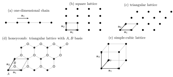
Five direct-space examples. Black and open circles in the honeycomb panel denote the $A$ and $B$ motif sites. The honeycomb sites do not form a Bravais lattice: the translation lattice is triangular, and each primitive cell contains both sites. Bonds are geometric guides, not part of the definition of a lattice.

One-dimensional chain

Choose

$$\mathbf a_1=a\hat{\mathbf x}, \qquad a>0.$$

Then

$$\Lambda = \{na\hat{\mathbf x}\mid n\in\mathbb Z\}, \qquad \Omega_{\mathrm c}=a.$$

A monatomic chain has one motif site, $\tau_1=0$. Each site has two nearest neighbors in the infinite chain, so its coordination number is $z=2$. A dimerized chain can use the same underlying spacing with alternating bonds, or it can use a doubled translation period $2a$ with a two-site motif. Which description is appropriate depends on the symmetry of the Hamiltonian, not only on the plotted points.

Square lattice

Take

$$\mathbf a_1=a(1,0), \qquad \mathbf a_2=a(0,1).$$

The primitive area and monatomic nearest-neighbor coordination are

$$\Omega_{\mathrm c}=a^2, \qquad z=4.$$

The square Bravais lattice has fourfold rotations about a lattice point. A motif can reduce that point symmetry even while preserving every translation.

Triangular lattice

A standard primitive basis is

$$\begin{aligned} \mathbf a_1&=a(1,0),\\ \mathbf a_2&=a \left( \frac12,\frac{\sqrt3}{2} \right). \end{aligned}$$

Its primitive area is

$$\Omega_{\mathrm c} = \frac{\sqrt3}{2}a^2.$$

For one site per cell, the six vectors

$$\pm\mathbf a_1, \qquad \pm\mathbf a_2, \qquad \pm(\mathbf a_2-\mathbf a_1)$$

form the nearest-neighbor shell, so $z=6$. In two-dimensional crystallography this Bravais type is called hexagonal; “triangular lattice” describes the visible point net and avoids confusion with the non-Bravais honeycomb structure.

Honeycomb structure

Use the same triangular Bravais lattice and attach two sites:

$$\boldsymbol\tau_A=\mathbf0, \qquad \boldsymbol\tau_B = \frac{\mathbf a_1+\mathbf a_2}{3}.$$

Here $a$ is the length of a primitive Bravais translation. The nearest-neighbor bond length is

$$d=\frac{a}{\sqrt3}.$$

The full site set is

$$\mathcal H = \Lambda \cup \bigl(\Lambda+\boldsymbol\tau_B\bigr).$$

Translations in $\Lambda$ preserve the $A$ and $B$ sublattices separately. A displacement from $A$ to $B$ is not a symmetry translation: translating twice by $\boldsymbol\tau_B$ produces the coset $\Lambda+2\boldsymbol\tau_B$, which is neither $\Lambda$ nor $\Lambda+\boldsymbol\tau_B$. Thus the honeycomb structure is a triangular Bravais lattice with a two-site motif, not a sixth two-dimensional Bravais type.

Graphene realizes this geometry with carbon atoms, while hexagonal boron nitride places different species on the two motif sites. The same positions therefore do not imply the same sublattice symmetry or electronic Hamiltonian.

Simple-cubic lattice

Choose

$$\begin{aligned} \mathbf a_1&=a(1,0,0),\\ \mathbf a_2&=a(0,1,0),\\ \mathbf a_3&=a(0,0,1). \end{aligned}$$

Then

$$\Omega_{\mathrm c}=a^3, \qquad z=6$$

for a monatomic nearest-neighbor geometry. Simple cubic, body-centered cubic, and face-centered cubic are three different Bravais types. The latter two are often drawn using cubic conventional cells that contain two and four primitive cells, respectively.

Physical Crystal Examples

The same lattice-plus-motif language handles familiar structures:

Structure	Translation lattice	Motif statement
monatomic face-centered cubic metal	face-centered cubic	one atom associated with each primitive cell
body-centered cubic elemental phase	body-centered cubic	one atom per primitive cell
graphene	two-dimensional triangular	two carbon sites, $A$ and $B$
hexagonal boron nitride layer	two-dimensional triangular	boron and nitrogen occupy different motif sites
diamond structure	face-centered cubic	two identical atoms displaced along a body diagonal
rock-salt structure	face-centered cubic	two interpenetrating ionic sublattices

Actual materials can change structure with temperature, pressure, composition, strain, or substrate. A structure label should therefore be understood as a statement about a specified phase and set of conditions.

Periodicity is not the same as crystallinity

An optical lattice can impose

$$V(\mathbf r+\mathbf R)=V(\mathbf r)$$

without the atoms spontaneously forming a rigid solid. Optical Lattices explains this controlled realization.

Conversely, a self-organized crystal is a phase of matter. In an ideal infinite system, crystalline order breaks continuous translations down to a discrete subgroup. The order is diagnosed through correlation functions and Bragg scaling, not merely by drawing particles near regular sites. See Long-Range Order for the many-body criterion.

Neighbor Shells, Bonds, and Models

The lattice determines displacement vectors between translation-equivalent cells. It does not by itself determine which sites are chemically bonded, which orbitals overlap appreciably, or which couplings belong in an effective Hamiltonian.

For motif sites $\alpha$ and $\beta$, a relative displacement has the form

$$\boldsymbol\delta_{\alpha\beta}(\mathbf R) = \mathbf R + \boldsymbol\tau_\alpha - \boldsymbol\tau_\beta.$$

Neighbor shells group these vectors by length, possibly refined by point-group symmetry. A tight-binding representation can then assign amplitudes

$$t_{\alpha\beta}(\mathbf R) = \left\langle \mathbf R,\alpha \middle| H \middle| \mathbf0,\beta \right\rangle.$$

Translation symmetry makes the amplitude depend on the cell difference rather than on two absolute cell labels. It does not require all geometrically equal distances to carry the same amplitude if the orbitals, species, magnetic order, or environment differ.

Coordination number is therefore model-dependent unless the neighbor criterion is stated. The values $z=2,4,6,3,6$ quoted for the chain, square, triangular, honeycomb, and simple-cubic examples refer to the nearest sites of the ideal monatomic or two-sublattice geometry.

Finite Samples and Boundary Conditions

An infinite lattice is a mathematical limit. A finite supercell with $N_i$ primitive translations along direction $i$ contains

$$N_{\mathrm c} = \prod_{i=1}^{d}N_i$$

primitive cells. With $q$ structural sites and $n_{\mathrm{orb}}$ retained orbitals per site, a simple localized one-particle basis has

$$\dim\mathcal H_1 = N_{\mathrm c}\,q\,n_{\mathrm{orb}}$$

states before additional spin, Nambu, flavor, or gauge redundancy is included.

Periodic boundary conditions identify

$$\mathbf R \sim \mathbf R+N_i\mathbf a_i.$$

The finite translation group becomes

$$\mathbb Z_{N_1} \times\cdots\times \mathbb Z_{N_d}.$$

This restores exact translation symmetry on a finite computational domain and leads to a discrete momentum mesh. It removes physical surfaces, however. Open boundaries retain edges and surface coordination changes but generally break translations near the boundary.

Boundary Conditions on Lattices develops finite many-body geometries, while Periodic Boundary Conditions gives the one-dimensional wave-mechanics foundation.

Thermodynamic-limit caution

For short-range bulk observables away from criticality, boundary contributions often scale like surface area while bulk contributions scale like volume. That heuristic does not justify discarding boundaries universally. Gapless modes, long-range interactions, topological boundary states, electrostatics, and transport contacts can keep boundary physics observable even in large samples.

Fractional Coordinates and Computational Geometry

The lattice matrix $A$ converts fractional coordinates $\boldsymbol\xi$ to Cartesian coordinates:

$$\mathbf r=A\boldsymbol\xi.$$

A motif position is commonly stored as

$$\boldsymbol\tau_\alpha = A\boldsymbol\xi_\alpha, \qquad 0\leq\xi_{\alpha i}<1.$$

The direct-space metric in fractional coordinates is

$$g=A^{\mathsf T}A,$$

so

$$|\mathbf r-\mathbf r'|^2 = \bigl(\boldsymbol\xi-\boldsymbol\xi'\bigr)^{\mathsf T} g \bigl(\boldsymbol\xi-\boldsymbol\xi'\bigr).$$

This formula matters for nonorthogonal cells. Componentwise wrapping of fractional differences into $[-1/2,1/2)$ does not always find the nearest periodic image in a strongly skewed cell. Robust neighbor searches compare an adequate set of translated images or use a lattice-reduction algorithm.

A reproducible structure file or simulation report should state:

• the ordered lattice vectors and their units;
• whether vectors are rows or columns;
• Cartesian or fractional motif coordinates;
• the origin choice;
• species, occupancies, and site labels;
• boundary conditions and supercell matrix;
• whether reported bonds are inferred geometrically or supplied explicitly.

Changing the primitive basis by $A'=AM$ also changes fractional coordinates:

$$\boldsymbol\xi' = M^{-1}\boldsymbol\xi.$$

Cartesian positions and physical observables remain unchanged when the motif and all tensor components are transformed consistently.

From Ionic Positions to a Periodic Hamiltonian

In an electronic-structure problem, nuclei are not literally fixed classical points. The common starting point is a scale-separated description in which equilibrium nuclear positions define a reference structure and electronic motion is solved conditionally on nuclear coordinates. Born–Oppenheimer Scale Separation owns that approximation.

Write an equilibrium nuclear position as

$$\mathbf R_{\ell\alpha}^{(0)} = \mathbf R_\ell+\boldsymbol\tau_\alpha.$$

The actual operator or instantaneous coordinate is more accurately represented by

$$\mathbf R_{\ell\alpha} = \mathbf R_{\ell\alpha}^{(0)} + \mathbf u_{\ell\alpha},$$

where $\mathbf u_{\ell\alpha}$ is a displacement. Setting every displacement to zero defines the ideal static lattice. Keeping small collective displacements leads to phonons; large, anharmonic, or topological distortions require more.

The periodic ionic reference can generate an electronic potential

$$V_{\mathrm{ion}}(\mathbf r+\mathbf R) = V_{\mathrm{ion}}(\mathbf r),$$

but an effective one-electron Hamiltonian may also contain self-consistent fields, spin-orbit coupling, magnetic order, or nonlocal terms. The correct symmetry is the symmetry of the full Hamiltonian, not of one term considered in isolation.

Band Structure Workflows takes this declared crystal and magnetic structure into a reproducible electronic-structure calculation, recording the cell choice, coordinates, species, charge, boundary idealization, and structure provenance. This page retains the direct-space definitions themselves.

What Diffraction Measures

A periodic density admits a Fourier series over a discrete set of reciprocal vectors:

$$\rho(\mathbf r) = \sum_{\mathbf G} \rho_{\mathbf G} e^{i\mathbf G\cdot\mathbf r}.$$

The next article derives which $\mathbf G$ are allowed from the condition

$$e^{i\mathbf G\cdot\mathbf R}=1.$$

For a motif, the amplitude contains a basis-dependent factor of the form

$$F(\mathbf G) = \sum_{\alpha} f_\alpha(\mathbf G) e^{-i\mathbf G\cdot\boldsymbol\tau_\alpha}.$$

Peak positions primarily reveal the translation lattice and its metric. Peak intensities, systematic absences, and probe dependence contain information about the motif, species, form factors, displacements, and correlations. A lattice cannot generally be reconstructed from a photograph of a few peaks without indexing choices and structural modeling.

An infinite perfect lattice gives ideal reciprocal-space delta peaks. Finite size, thermal motion, defects, domains, strain, and instrumental resolution broaden or attenuate them. Structure Factors develops the correlation-function observable, and Electron Diffraction gives an experimental route to crystalline periodicity.

What the Ideal Lattice Approximation Ignores

The ideal lattice is a reference configuration, not a complete material model.

Omitted feature	What changes physically
zero-point and thermal motion	atomic positions fluctuate; Bragg intensity is reduced and phonons appear
anharmonicity	normal modes interact; thermal expansion and finite lifetimes arise
vacancies and interstitials	translation symmetry is locally broken and carrier or phonon scattering changes
substitutional disorder	site energies, masses, and local environments vary
dislocations and strain	lattice vectors become local fields; topology and elasticity enter
surfaces and interfaces	coordination, electrostatics, and allowed states differ from the bulk
domains, twins, and grain boundaries	several orientations or order-parameter choices coexist
incommensurate order	no finite common primitive cell may exist
quasicrystalline order	sharp diffraction can occur without ordinary translation periodicity
finite correlation length	periodic order is approximate rather than asymptotically long-ranged

Whether an omission is controlled depends on the observable and scale. A weak concentration of defects may barely change a band dispersion yet dominate low-temperature resistivity. Small atomic displacements can be negligible for static geometry but essential for heat capacity and superconducting pairing. A surface can be irrelevant to a bulk equation of state and decisive for photoemission or a topological phase.

A useful approximation audit

Before applying a perfect-lattice model, ask:

1. Which translation group is assumed?
2. Is it imposed externally or selected spontaneously?
3. What motif and internal degrees of freedom are retained?
4. Which deviations from periodicity are small in the observable of interest?
5. Are boundaries, disorder, or fluctuations being averaged, neglected, or modeled?
6. What experiment determines the structural parameters?

Calling a Hamiltonian “on a lattice” answers none of these questions by itself.

Common Mistakes

Mistake	Correction
identifying every visible site with a Bravais-lattice point	find the smallest pure translations that preserve the entire decorated structure
calling honeycomb a Bravais lattice	use a triangular Bravais lattice with a two-site motif
assuming primitive vectors are unique	primitive bases are related by unimodular integer transformations
choosing any two independent lattice vectors as primitive	their integer transformation must have determinant $\pm1$
treating a conventional cell as primitive	compare its volume with the primitive-cell volume or inspect centering translations
saying a primitive cell “contains one atom”	it contains one lattice point by convention but may carry any motif
confusing structural and orbital bases	list atomic sites and retained Hilbert-space states separately
inferring bonds from the lattice alone	state the neighbor rule or Hamiltonian matrix elements
believing electrons occupy only lattice points	continuum electrons remain continuous unless a lattice model is introduced
treating periodic boundaries as a real surface	periodic boundaries remove the surface and change the finite translation group
assuming sharp diffraction proves a simple periodic crystal	incommensurate and quasiperiodic structures require more careful analysis

Exercises

Exercise 1: prove the group structure

Let

$$\Lambda = \left\{ \sum_{i=1}^{d}n_i\mathbf a_i \mid n_i\in\mathbb Z \right\}$$

with linearly independent $\mathbf a_i$. Prove that $\Lambda$ is an abelian group under addition and that the coefficient map $\mathbb Z^d\to\Lambda$ is an isomorphism.

Solution

If $\mathbf R=A\mathbf n$ and $\mathbf R'=A\mathbf n'$ with integer vectors $\mathbf n,\mathbf n'$, then

$$\mathbf R+\mathbf R' = A(\mathbf n+\mathbf n') \in\Lambda.$$

The zero vector is $A\mathbf0$, and the inverse of $A\mathbf n$ is $A(-\mathbf n)$. Associativity and commutativity are inherited from vector addition.

Define $\phi:\mathbb Z^d\to\Lambda$ by $\phi(\mathbf n)=A\mathbf n$. It is surjective by the definition of $\Lambda$. If $\phi(\mathbf n)=\phi(\mathbf n')$, then

$$A(\mathbf n-\mathbf n')=\mathbf0.$$

Linear independence of the columns of $A$ implies $\mathbf n=\mathbf n'$, so $\phi$ is injective. It also preserves addition, hence it is a group isomorphism.

Exercise 2: primitive or doubled?

For a square lattice with primitive matrix $A=(\mathbf a_1\ \mathbf a_2)$, consider

$$\begin{aligned} \mathbf b_1&=2\mathbf a_1+\mathbf a_2,\\ \mathbf b_2&=\mathbf a_1+\mathbf a_2. \end{aligned}$$

Do $\mathbf b_1,\mathbf b_2$ form a primitive basis? Repeat for

$$\mathbf c_1=\mathbf a_1+\mathbf a_2, \qquad \mathbf c_2=\mathbf a_1-\mathbf a_2.$$

Solution

For the first pair,

$$B = A \begin{pmatrix} 2&1\\ 1&1 \end{pmatrix},$$

and the integer matrix has determinant $1$. It is unimodular, so $\mathbf b_1,\mathbf b_2$ are primitive and span the same lattice.

For the second pair,

$$C = A \begin{pmatrix} 1&1\\ 1&-1 \end{pmatrix},$$

whose determinant is $-2$. The cell area is $2a^2$, and the generated points satisfy a parity restriction on their original integer coordinates. The pair spans an index-two sublattice, not the full square lattice.

Exercise 3: triangular geometry

For

$$\mathbf a_1=a(1,0), \qquad \mathbf a_2=a \left( \frac12,\frac{\sqrt3}{2} \right),$$

compute the primitive area and show that the six listed nearest-neighbor vectors all have length $a$.

Solution

The determinant is

$$\det \begin{pmatrix} a&a/2\\ 0&\sqrt3a/2 \end{pmatrix} = \frac{\sqrt3}{2}a^2.$$

Clearly $|\mathbf a_1|=|\mathbf a_2|=a$. Also

$$|\mathbf a_2-\mathbf a_1|^2 = a^2 \left[ \left(-\frac12\right)^2 + \left(\frac{\sqrt3}{2}\right)^2 \right] = a^2.$$

Changing signs preserves length, giving six vectors of length $a$. No nonzero integer combination is shorter, so these form the nearest-neighbor shell.

Exercise 4: why honeycomb is non-Bravais

Let

$$\mathcal H = \Lambda \cup \bigl(\Lambda+\boldsymbol\tau\bigr), \qquad \boldsymbol\tau = \frac{\mathbf a_1+\mathbf a_2}{3}.$$

Show that no pure translation taking an $A$ site to a $B$ site preserves $\mathcal H$.

Solution

Any displacement taking an $A$ site to a $B$ site is congruent to $\boldsymbol\tau$ modulo $\Lambda$. It is therefore enough to test translation by $\boldsymbol\tau$:

$$\mathcal H+\boldsymbol\tau = \bigl(\Lambda+\boldsymbol\tau\bigr) \cup \bigl(\Lambda+2\boldsymbol\tau\bigr).$$

The first coset is part of $\mathcal H$. Equality would require the second coset to equal $\Lambda$. That would mean

$$2\boldsymbol\tau = \frac{2}{3}\mathbf a_1 + \frac{2}{3}\mathbf a_2 \in\Lambda,$$

which is false because its primitive coordinates are not integers. It also cannot equal $\Lambda+\boldsymbol\tau$, because their difference $\boldsymbol\tau$ is not in $\Lambda$. Thus a pure translation cannot interchange the two sublattices. The primitive translations are those of the triangular $\Lambda$, and the motif has two sites.

Exercise 5: finite-cell counting

A periodic honeycomb supercell has $N_1N_2$ primitive cells. Retain one spinful orbital on each of its two structural sites. How many one-particle basis states are there? How many electrons correspond to one electron per site?

Solution

There are two sites per primitive cell and two spin states per orbital, so

$$\dim\mathcal H_1 = 4N_1N_2.$$

One electron per site gives

$$N_{\mathrm e} = 2N_1N_2.$$

This is half filling of the spin-resolved one-particle basis. The statement does not imply that every site is exactly singly occupied in an itinerant quantum state; it fixes only the total particle number.

Exercise 6: periodicity of a motif density

Starting from

$$\rho(\mathbf r) = \sum_{\mathbf R,\alpha} f_\alpha \bigl( \mathbf r-\mathbf R-\boldsymbol\tau_\alpha \bigr),$$

prove $\rho(\mathbf r+\mathbf R_0)=\rho(\mathbf r)$ for every $\mathbf R_0\in\Lambda$. Identify the step that fails for a single vacancy.

Solution

Translate the argument:

$$\rho(\mathbf r+\mathbf R_0) = \sum_{\mathbf R,\alpha} f_\alpha \bigl( \mathbf r-(\mathbf R-\mathbf R_0)-\boldsymbol\tau_\alpha \bigr).$$

Because $\Lambda$ is a group, the map

$$\mathbf R\longmapsto\mathbf R-\mathbf R_0$$

is a bijection of $\Lambda$. Relabeling the dummy lattice vector therefore recovers $\rho(\mathbf r)$.

A vacancy removes one selected term, so the translated sum no longer has the same set of terms. The relabeling argument fails at the missing cell even though the underlying reference lattice remains useful.

Exercise 7: approximation audit

A calculation predicts a perfect-crystal band gap but an experiment measures a broad in-gap optical tail. Give four distinct departures from the ideal lattice that could contribute, and state what additional evidence would help distinguish them.

Solution

Possible mechanisms include:

• substitutional disorder or vacancies creating localized in-gap states;
• strain inhomogeneity shifting the local band edges;
• surfaces or interfaces supporting states absent from the bulk model;
• thermal or zero-point lattice motion enabling phonon-assisted absorption;
• domains or secondary structural phases with different gaps;
• an incorrect motif, magnetic order, or interaction approximation in the nominally perfect model.

Useful discriminants include temperature dependence, thickness or surface sensitivity, spatially resolved spectroscopy, diffraction and pair-distribution measurements, controlled annealing or irradiation, polarization selection rules, and comparison across samples with quantified composition. The observation alone does not identify “disorder” as a unique cause.

Connections

• The chapter gateway selects the shortest route from direct-space structure to reciprocal geometry, Bloch sectors, band models, or band-derived outputs.
• Quantum Matter places the lattice description inside the hierarchy from microscopic structure to observables.
• Quantum Matter Map shows when direct-space structure, reciprocal space, quasiparticles, and response are the appropriate levels of description.
• Crystalline Symmetry Preview connects lattice translations to point groups, space groups, and Bloch phases.
• Structure Factors gives the correlation-function language used by scattering probes.
• Lattice Models Overview explains how a structural or emergent lattice becomes a many-body Hamiltonian.
• Reciprocal Lattice is the next technical step: it constructs the wavevectors whose phases are invariant under every $\mathbf R\in\Lambda$.

References

• M. I. Aroyo, ed., International Tables for Crystallography A: Space-Group Symmetry, 6th ed. (Wiley, 2016), especially the tables of two- and three-dimensional Bravais types.
• N. W. Ashcroft and N. D. Mermin, Solid State Physics (Holt, Rinehart and Winston, 1976), Chapters 4–7.
• P. M. Chaikin and T. C. Lubensky, Principles of Condensed Matter Physics (Cambridge University Press, 1995), Chapters 4–5.
• International Union of Crystallography, “Unit cell,” Online Dictionary of Crystallography, accessed 2026-07-26.
• C. Kittel, Introduction to Solid State Physics, 8th ed. (Wiley, 2004), Chapters 1–2.
• M. P. Marder, Condensed Matter Physics, 2nd ed. (Wiley, 2010), Chapters 1–3.
• J. F. Nye, Physical Properties of Crystals (Oxford University Press, 1985), Chapters 1–3.
• B. Souvignier, “A general introduction to space groups,” International Tables for Crystallography A, Chapter 1.3, 22–41 (2016), doi:10.1107/97809553602060000921.
• G. L. Squires, Introduction to the Theory of Thermal Neutron Scattering, 3rd ed. (Cambridge University Press, 2012), Chapters 1–3.
• P. R. Wallace, “The Band Theory of Graphite,” Physical Review 71, 622–634 (1947), doi:10.1103/PhysRev.71.622.
• B. E. Warren, X-Ray Diffraction (Dover, 1990), Chapters 1–4.