Magnetic Anisotropy

Magnetic anisotropy is the dependence of a magnetic system’s free energy on the orientation of its order parameter relative to the crystal, sample, interfaces, strain, or other fixed spatial structure. An easy axis is an orientation that minimizes this free energy; an easy plane is a continuous set of minimizing directions within a plane. The corresponding maxima are hard directions.

Anisotropy turns a rotationally symmetric magnetic model into a material. It selects the direction of a ferromagnetic magnetization or antiferromagnetic Néel vector, gaps some spin-wave modes, controls coherent-rotation fields, contributes to domain-wall width and energy, and competes with dipolar and Dzyaloshinskii–Moriya interactions to organize textures.

The phrase covers several mechanisms that must not be conflated:

• magnetocrystalline anisotropy, generated when spin–orbit coupling ties spin and orbital moments to crystal symmetry;
• single-ion anisotropy, a local low-energy representation of crystal-field and spin–orbit physics;
• anisotropic exchange, including symmetric exchange and antisymmetric Dzyaloshinskii–Moriya coupling;
• shape anisotropy, the orientation dependence of magnetostatic self-energy;
• surface and interface anisotropy, allowed because translation and inversion symmetries differ from the bulk;
• magnetoelastic anisotropy, generated by strain and magnetostriction.

Spin–Orbit Coupling in Solids owns the microscopic spin–orbital bridge. Exchange Interactions owns the exchange-tensor decomposition and bond conventions. This page owns their orientation-dependent material free energy and the route from anisotropy constants to observables and texture scales.

Required background. Spin–Orbit Coupling in Solids supplies the microscopic spin–orbital bridge, while Exchange Interactions supplies exchange-tensor and bond conventions.

Helpful background. Ferromagnetism and Antiferromagnetism provide the uniform and staggered order-parameter branches.

Convention ledger

Before quoting an anisotropy constant, state:

• the orientation variable: magnetization $\mathbf M$, unit vector $\mathbf m=\mathbf M/M_s$, Néel vector $\mathbf l$, or a pseudospin axis;
• the reference direction and angle convention;
• whether the quantity is energy per volume, area, magnetic ion, formula unit, or computational cell;
• whether it is an internal-energy difference at zero temperature or a free-energy difference at finite temperature;
• whether shape, surface, strain, applied field, and dipolar contributions have been included;
• whether the field variable is $\mathbf H$ or $\mathbf B$ and whether SI or Gaussian demagnetizing factors are used.

We use SI units. For ellipsoidal samples the dimensionless principal demagnetizing factors obey

$$N_x+N_y+N_z=1.$$

Some Gaussian-unit tables instead normalize their sum to $4\pi$. Mixing those conventions produces an error by $4\pi$.

For a ferromagnet in zero applied field, reversing all moments is a time-reversal-related state. The orientation energy therefore satisfies

$$f_{\mathrm{an}}(\mathbf m) = f_{\mathrm{an}}(-\mathbf m)$$

unless another fixed time-reversal-odd object is present. Crystal anisotropy expansions consequently begin with even powers of $\mathbf m$. Dzyaloshinskii–Moriya terms can be linear in spatial gradients while remaining even under simultaneous reversal of every spin.

Symmetry before coefficients

At quadratic order, the most general orientation energy of a unit axial vector is

$$f_{\mathrm{an}}^{(2)} = \mathbf m^{\mathsf T} \mathsf K \mathbf m,$$

where only the symmetric part of $\mathsf K$ contributes. Adding a multiple of the identity shifts every orientation by the same constant because $\mathbf m^2=1$. The physically relevant quadratic anisotropy is therefore the traceless part.

For every spatial symmetry represented by $R$, the tensor must satisfy

$$R\mathsf K R^{\mathsf T} = \mathsf K.$$

Diagonalizing $\mathsf K$ identifies its principal directions. In a uniaxial environment, two eigenvalues coincide and the remaining eigenvector defines the symmetry axis. In a fully cubic environment, symmetry forces $\mathsf K$ to be proportional to the identity, so quadratic orientation dependence is only a constant. Cubic magnetocrystalline anisotropy begins at fourth order.

This invariant method is more reliable than guessing an “anisotropy axis” from a drawing. For an antiferromagnet, apply the magnetic space group to the Néel vector and any weak ferromagnetic moment together. A crystallographic axis need not be magnetically easy, and symmetry determines allowed terms rather than their signs or magnitudes.

Easy axes, planes, and cones

Let $\theta$ be the angle from a uniaxial crystal axis $\hat{\mathbf z}$. A common expansion is

$$f_u(\theta,\phi) = K_1\sin^2\theta + K_2\sin^4\theta + f_\parallel(\theta,\phi),$$

where $f_\parallel$ contains symmetry-allowed in-plane harmonics. With $K_2=0$ in this convention:

• $K_1>0$ gives an easy axis along $\pm\hat{\mathbf z}$;
• $K_1<0$ gives an easy plane perpendicular to $\hat{\mathbf z}$.

Another common convention writes $K\cos^2\theta$, reversing the verbal sign rule. A sign without the defining equation is not useful.

Higher-order terms can create an easy cone. Setting

$$x=\sin^2\theta, \qquad 0\le x\le1,$$

gives

$$f_u(x)=K_1x+K_2x^2.$$

For $K_2>0$ and

$$-2K_2<K_1<0,$$

the minimum lies at

$$\sin^2\theta_0 = -\frac{K_1}{2K_2}.$$

Thus the sign of one coefficient need not identify the actual easy direction.

Cubic crystals

For direction cosines

$$\alpha_i = \mathbf m\cdot\hat{\mathbf e}_i, \qquad \sum_i\alpha_i^2=1,$$

the leading cubic anisotropy is

$$\begin{aligned} f_{\mathrm{cub}} = & K_1 \left( \alpha_1^2\alpha_2^2 + \alpha_2^2\alpha_3^2 + \alpha_3^2\alpha_1^2 \right) \\ &+ K_2 \alpha_1^2\alpha_2^2\alpha_3^2 + \cdots . \end{aligned}$$

The high-symmetry values are

$$\begin{array}{c|c} \text{direction} & f_{\mathrm{cub}} \\ \hline \langle100\rangle & 0 \\ \langle110\rangle & K_1/4 \\ \langle111\rangle & K_1/3+K_2/27 \end{array}$$

and the minimum determines the easy family. When $K_2$ is negligible, $K_1>0$ favors $\langle100\rangle$ and $K_1<0$ favors $\langle111\rangle$. Large higher-order terms can change that simple rule.

Anisotropy field

For a single-domain uniaxial ferromagnet with a transverse field,

$$f(\theta) = K_{\mathrm{eff}}\sin^2\theta - \mu_0M_sH\sin\theta ,$$

where $K_{\mathrm{eff}}>0$, coherent rotation reaches the hard direction at

$$H_K = \frac{2K_{\mathrm{eff}}}{\mu_0M_s}.$$

Equivalently,

$$\mu_0H_K = \frac{2K_{\mathrm{eff}}}{M_s}.$$

$H_K$ is not generally the coercive field. Coercivity depends on nucleation, defects, pinning, thermal activation, domain-wall motion, sweep protocol, and sample history. Equality occurs only in restricted coherent-rotation models.

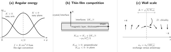
Three levels of anisotropy modeling. Left: the sign rule belongs to a declared angular-energy convention. Center: perpendicular crystal and interface anisotropy competes with the thin film’s demagnetizing energy. Right: exchange and effective anisotropy set the wall scale $\Delta=\sqrt{A/K_{\mathrm{eff}}}$, while Dzyaloshinskii–Moriya coupling selects chirality and changes the wall energy in the ideal one-dimensional model.

Crystal-field and spin–orbit mechanisms

Electrostatic crystal fields act primarily on orbital charge distributions. Spin–orbit coupling then ties those orbitals to spin or total angular momentum, producing an orientation-dependent energy. Because the effect compares nearly equal total energies, its scale can be much smaller than the spin–orbit matrix elements that generate it.

Single-ion representation

For a dimensionless local spin $s\ge1$, a frequently used effective Hamiltonian is

$$H_{\mathrm{SIA}} = D s_z^2 + E \left( s_x^2-s_y^2 \right) + \cdots .$$

With this sign convention, $D<0$ favors large $|m_S|$ and is easy-axis-like, while $D>0$ favors small $|m_S|$ and is easy-plane-like. The $E$ term removes in-plane equivalence.

For $s=1/2$,

$$s_x^2 = s_y^2 = s_z^2 = \frac{1}{4}I.$$

The quadratic onsite term is therefore a constant and cannot split an isolated Kramers doublet at zero field. An effective spin-$1/2$ can still have an anisotropic $g$ tensor and anisotropic exchange. A reported zero-field $Ds_z^2$ splitting for a genuine two-state Kramers system indicates that additional states, time-reversal breaking, or an inappropriate effective model have been hidden.

For rare-earth and actinide ions, the crystal field within a fixed $J$ multiplet is often expanded in Stevens operators:

$$H_{\mathrm{CF}} = \sum_{k,q} B_k^q O_k^q(\mathbf J).$$

Only terms allowed by the site point group survive. The coefficients depend on ligand geometry, screening, covalency, and radial matrix elements. A non-Kramers ion can acquire a singlet or split non-Kramers doublet under lower symmetry, whereas a Kramers doublet remains degenerate until time reversal is broken.

Itinerant magnetocrystalline anisotropy

In an itinerant magnet, rotating the magnetization changes spin–orbit hybridization throughout the occupied band structure. In second-order perturbation theory,

$$E_{\mathrm{SO}}^{(2)}(\hat{\mathbf n}) = \sum_{\substack{o\ \mathrm{occ}\\u\ \mathrm{unocc}}} \frac{ \left| \langle u| H_{\mathrm{SO}}(\hat{\mathbf n}) |o\rangle \right|^2 }{ \varepsilon_o-\varepsilon_u }.$$

The magnetocrystalline anisotropy energy is a difference such as

$$K_{\hat{\mathbf n}_1-\hat{\mathbf n}_2} = E(\hat{\mathbf n}_1) - E(\hat{\mathbf n}_2).$$

Near-degenerate occupied and unoccupied states can dominate because of the small denominator. This makes anisotropy sensitive to band filling, strain, interfaces, correlation treatment, and numerical convergence.

Under a restricted set of assumptions—large exchange splitting, weak spin–orbit coupling, negligible spin-flip terms, and an appropriate tight-binding description—the Bruno relation connects anisotropy to orbital-moment anisotropy:

$$K_{\hat{\mathbf n}_1-\hat{\mathbf n}_2} \simeq -\frac{\xi}{4\mu_{\mathrm B}} \left[ m_L(\hat{\mathbf n}_1) - m_L(\hat{\mathbf n}_2) \right].$$

It is a useful diagnostic, not an identity for arbitrary multiorbital, strongly relativistic, antiferromagnetic, or correlated materials.

Magnetoelastic coupling

For a cubic ferromagnet, a leading magnetoelastic energy is

$$\begin{aligned} f_{\mathrm{me}} = & B_1 \left( \epsilon_{xx}\alpha_x^2 + \epsilon_{yy}\alpha_y^2 + \epsilon_{zz}\alpha_z^2 \right) \\ &+ 2B_2 \left( \epsilon_{xy}\alpha_x\alpha_y + \epsilon_{yz}\alpha_y\alpha_z + \epsilon_{zx}\alpha_z\alpha_x \right). \end{aligned}$$

Strain can therefore change the easy direction even if the unstrained crystal constants are fixed. Conversely, rotating the magnetization can change the equilibrium strain: magnetostriction and magnetoelastic anisotropy are reciprocal descriptions of the same coupling.

Surfaces and interfaces

At a surface, missing neighbors, altered hybridization, relaxation, electric fields, and reduced point-group symmetry permit anisotropy terms absent or equivalent in the bulk. A leading surface contribution is an energy per area,

$$\frac{F_s}{A} = K_s \left[ 1- (\mathbf m\cdot\hat{\mathbf n})^2 \right],$$

where positive $K_s$ favors the surface normal $\hat{\mathbf n}$ in this convention. For two inequivalent interfaces, the film contribution is

$$\frac{ K_s^{\mathrm{top}} + K_s^{\mathrm{bottom}} }{t},$$

not automatically $2K_s/t$.

The atomic-scale origin may be described through broken-bond pair anisotropy, interface-modified orbital moments, strain, charge transfer, or hybridization with a heavy adjacent layer. Thickness scaling can separate area-like and volume-like terms only over a range where the structure, magnetization, and interface chemistry remain comparable. Voltage control of anisotropy can reflect electrostatic occupation changes, ionic motion, piezoelectric strain, or redox chemistry; a gate dependence alone does not identify which mechanism operates.

Shape anisotropy and demagnetizing fields

A nonuniform magnetization produces a magnetostatic field $\mathbf H_d$ satisfying

$$\boldsymbol{\nabla}\times\mathbf H_d=0, \qquad \boldsymbol{\nabla}\cdot \left( \mathbf H_d+\mathbf M \right) = 0.$$

Writing $\mathbf H_d=-\boldsymbol{\nabla}\Phi_m$ gives

$$\nabla^2\Phi_m = \boldsymbol{\nabla}\cdot\mathbf M.$$

The magnetostatic self-energy can be expressed as

$$\begin{aligned} E_d &= -\frac{\mu_0}{2} \int_V \mathbf M\cdot\mathbf H_d\, \mathrm d^3r \\ &= \frac{\mu_0}{2} \int_{\mathrm{all\ space}} |\mathbf H_d|^2\, \mathrm d^3r . \end{aligned}$$

For a uniformly magnetized ellipsoid, the internal field is uniform:

$$\mathbf H_d = -\mathsf N\mathbf M.$$

Along the principal axes,

$$\frac{E_d}{V} = \frac{\mu_0}{2} \left( N_xM_x^2 + N_yM_y^2 + N_zM_z^2 \right).$$

The easiest shape direction has the smallest $N_i$. Useful limits are:

$$\begin{array}{c|ccc} \text{shape} & N_x & N_y & N_z \\ \hline \text{sphere} & 1/3 & 1/3 & 1/3 \\ \text{thin film, normal }z & 0 & 0 & 1 \\ \text{long needle, axis }z & 1/2 & 1/2 & 0 \end{array}$$

The film and needle entries are ideal infinite-aspect-ratio limits. For a finite rectangular prism, $\mathbf H_d$ is nonuniform and a single demagnetizing tensor is at best an averaged description tied to a specified magnetization state.

Perpendicular anisotropy in a film

Suppose a film has a volume magnetocrystalline contribution $K_v$, two equivalent interface contributions $K_s$ per area, thickness $t$, and uniform $M_s$. Taking positive $K$ to favor the film normal,

$$K_{\mathrm{eff}} = K_v + \frac{2K_s}{t} - \frac{\mu_0M_s^2}{2}.$$

$K_{\mathrm{eff}}>0$ favors perpendicular magnetization, whereas $K_{\mathrm{eff}}<0$ favors the film plane in the uniform approximation. The $1/t$ dependence is a useful interface diagnostic, but roughness, dead layers, asymmetric interfaces, thickness-dependent $M_s$, strain relaxation, and higher-order terms can spoil a straight-line extraction.

Shape anisotropy is often called a dipolar anisotropy. It is not a local crystal constant. A sample can reduce its magnetostatic energy by forming domains, so the direction observed in a multidomain image is not automatically the intrinsic uniform-state easy axis.

Anisotropic exchange and Dzyaloshinskii–Moriya coupling

A general bilinear pair interaction can be decomposed as

$$\begin{aligned} H_{ij} = & J_{ij}\, \mathbf s_i\cdot\mathbf s_j \\ &+ \mathbf D_{ij}\cdot \left( \mathbf s_i\times\mathbf s_j \right) \\ &+ \mathbf s_i\cdot \mathsf\Gamma_{ij} \mathbf s_j , \end{aligned}$$

where $\mathsf\Gamma_{ij}$ is symmetric and traceless. Reversing the declared bond orientation changes

$$\mathbf D_{ji} = -\mathbf D_{ij}.$$

An inversion center at the bond midpoint forces $\mathbf D_{ij}=0$. Other point-group operations constrain its allowed direction. Broken inversion is necessary but not sufficient for an arbitrary Dzyaloshinskii–Moriya vector.

For a uniform collinear state,

$$\mathbf s_i\times\mathbf s_j=0,$$

so Dzyaloshinskii–Moriya coupling does not by itself define the easy direction of that state. It favors canting and handed spatial variation. Symmetric anisotropic exchange can contribute directly to the energy of a collinear orientation.

Continuum invariants

For a unit magnetization field $\mathbf m(\mathbf r)$, a representative micromagnetic functional is

$$\begin{aligned} F[\mathbf m] = \int\mathrm d^3r\, \big[ & A \sum_i (\partial_i\mathbf m)^2 \\ &+ K_{\mathrm{eff}} (1-m_z^2) + f_{\mathrm D} + f_d \\ &- \mu_0M_s \mathbf H\cdot\mathbf m \big]. \end{aligned}$$

Here $A$ is exchange stiffness and $f_d$ denotes the nonlocal magnetostatic contribution. Two common Dzyaloshinskii–Moriya densities are

$$f_{\mathrm D}^{\mathrm{bulk}} = D\, \mathbf m\cdot \left( \boldsymbol{\nabla}\times\mathbf m \right)$$

for an isotropic chiral bulk crystal, and

$$f_{\mathrm D}^{\mathrm{int}} = D \left[ m_z\boldsymbol{\nabla}\cdot\mathbf m - (\mathbf m\cdot\boldsymbol{\nabla})m_z \right]$$

for an ideal interface with polar normal $\hat{\mathbf z}$. Their signs depend on coordinate and chirality conventions. Using a bulk invariant for an interface, or vice versa, gives the wrong texture.

From anisotropy to magnetic textures

Exchange penalizes rapid variation, anisotropy penalizes departure from preferred directions, magnetostatics rewards flux closure, and Dzyaloshinskii–Moriya coupling rewards a selected twist. Their competition creates domains, walls, spirals, bubbles, and skyrmions.

Exchange and anisotropy lengths

Two useful scales are

$$\ell_K = \sqrt{ \frac{A}{K_{\mathrm{eff}}} }, \qquad \ell_{\mathrm{ex}} = \sqrt{ \frac{2A}{\mu_0M_s^2} }.$$

$\ell_K$ compares exchange with uniaxial anisotropy; $\ell_{\mathrm{ex}}$ compares exchange with magnetostatic energy. They answer different questions and should not both be called “the exchange length” without definition.

For a one-dimensional $180^\circ$ wall with

$$\mathbf m = \left( \sin\theta,0,\cos\theta \right),$$

and energy per wall area

$$\sigma = \int_{-\infty}^{\infty} \left[ A(\theta')^2 + K_{\mathrm{eff}}\sin^2\theta \right] \mathrm dx,$$

the minimizing profile is

$$\theta(x) = 2\arctan \exp \left( \frac{x-X}{\Delta} \right), \qquad \Delta = \sqrt{ \frac{A}{K_{\mathrm{eff}}} }.$$

Its energy is

$$\sigma_0 = 4\sqrt{ AK_{\mathrm{eff}} }.$$

Some authors call $\Delta$ the wall width; others define a geometric width $\delta=\pi\Delta$. Numerical values should always state the convention.

For the favored Néel chirality in the ideal ultrathin interfacial model,

$$\sigma_{\mathrm{wall}} = 4\sqrt{ AK_{\mathrm{eff}} } - \pi|D|.$$

The nominal threshold at which this isolated-wall expression reaches zero is

$$D_c = \frac{4}{\pi} \sqrt{ AK_{\mathrm{eff}} }.$$

This is not a universal skyrmion-stability criterion. Dipolar fields, confinement, field, lattice discreteness, higher-order anisotropy, disorder, finite temperature, and the full competing phase diagram all matter.

Skyrmions and Magnetic Textures owns domain topology, vortices, skyrmion charge, detailed stability, dynamics, and experimental signatures. Here the texture formulas serve only to show how anisotropy enters the energetic ledger.

Bloch and Néel walls are distinguished by the plane in which $\mathbf m$ rotates. In a bulk uniaxial magnet, magnetostatic geometry often decides between them. At an inversion-asymmetric interface, Dzyaloshinskii–Moriya coupling can select a Néel wall and one handedness. Observing one wall type therefore constrains an energy competition; it does not measure one coefficient without the others.

Ferromagnets and antiferromagnets

In a ferromagnet, anisotropy acts on $\mathbf M$ and is often measured through torque, resonance, hard-axis saturation, or orientation-dependent total energy. Magnetostatic shape effects can be comparable to or larger than magnetocrystalline terms.

In a collinear antiferromagnet, the principal orientation variable is the Néel vector

$$\mathbf l = \frac{ \mathbf M_A-\mathbf M_B }{ 2M_0 }.$$

The net magnetization can be nearly zero while spin–orbit coupling still produces a substantial $f_{\mathrm{an}}(\mathbf l)$. Shape anisotropy of the net moment may then be weak, but dipolar coupling between sublattices, weak ferromagnetic canting, and surface moments can remain relevant.

Exchange and anisotropy fields also enter differently. In a simple two-sublattice easy-axis antiferromagnet with

$$H_A\ll H_E,$$

the spin-flop scale behaves schematically as

$$H_{\mathrm{sf}} \sim \sqrt{ 2H_EH_A }.$$

The large exchange field amplifies a modest anisotropy in the resonance and reorientation scales. Exact coefficients depend on field direction, sublattice moments, anisotropy terms, and convention.

Temperature and effective parameters

An anisotropy constant inferred at finite temperature is a free-energy coefficient after thermal electronic, spin, lattice, and possibly domain degrees of freedom have been integrated out. It need not equal a zero-temperature energy difference.

For localized single-ion anisotropy under restrictive assumptions, the Callen–Callen relation suggests

$$\frac{K_\ell(T)}{K_\ell(0)} \approx \left[ \frac{M(T)}{M(0)} \right]^{ \ell(\ell+1)/2 }.$$

For a leading second-rank uniaxial term this gives the familiar cubic power. The relation is not universal for itinerant magnets, two-ion anisotropy, antiferromagnets, interfaces, or temperatures near a phase transition. Competing terms with different temperature dependences can drive a spin-reorientation transition.

Energy barriers and switching

For a single-domain particle with two equivalent uniaxial minima and no applied field, the ideal coherent-rotation barrier is

$$\Delta E_0 = K_{\mathrm{eff}}V.$$

The dimensionless thermal-stability factor is

$$\mathcal S = \frac{ K_{\mathrm{eff}}V }{ k_{\mathrm B}T }.$$

In a simple Néel–Brown picture, the mean reversal time is approximately

$$\tau \sim \tau_0 \exp(\mathcal S),$$

with an attempt time $\tau_0$ determined by damping, curvature of the energy landscape, and field. This exponential sensitivity is why anisotropy is central to magnetic recording and nanomagnet stability. Spintronics develops how retention competes with spin-torque write current in device architectures.

Real particles can reverse by curling, edge nucleation, domain-wall propagation, or collective modes with barriers below $K_{\mathrm{eff}}V$. The relevant barrier is the lowest free-energy saddle compatible with geometry and observation time. A blocking temperature is therefore protocol dependent, not a thermodynamic phase boundary.

Experimental and computational inference

Torque and angular scans

The magnetic torque is

$$\boldsymbol{\tau} = -\frac{\partial F}{\partial\boldsymbol{\theta}},$$

where the derivative denotes rotation in the specified plane. For $f=K\sin^2\theta$,

$$\frac{\tau_\theta}{V} = -K\sin2\theta.$$

Angular harmonics identify allowed symmetry terms, but background torque from the holder, field misalignment, incomplete saturation, and demagnetizing geometry must be controlled.

Magnetometry and resonance

Hard-axis magnetization can estimate $H_K$ only if the sample rotates coherently or the domain process is modeled. Ferromagnetic resonance accesses derivatives of the free energy around equilibrium; converting resonance fields to $K_i$ requires the correct sample geometry, $M_s$, $g$ tensor, field orientation, and mode assignment.

Antiferromagnetic resonance, inelastic neutron scattering, and terahertz spectroscopy can infer anisotropy from mode gaps and field evolution. Spin Waves and Magnons explains why energies, intensities, polarization, and linewidths should be fitted together.

Magnetic imaging reveals domains and walls, not an anisotropy constant by itself. Extracting $A$, $K_{\mathrm{eff}}$, and $D$ from one measured wall width is underdetermined unless independent constraints and the appropriate wall model are supplied. X-ray magnetic circular dichroism can constrain spin and orbital moments, while linear dichroism can be sensitive to antiferromagnetic orientation; their sum rules, projection geometry, and multiplet assumptions must be stated.

First-principles calculations

A robust magnetocrystalline-anisotropy calculation should:

1. converge total-energy differences with respect to momentum mesh, basis, smearing, and self-consistency;
2. state whether it uses fully self-consistent energies, a force theorem, or a torque method;
3. use the same structure, electron number, and numerical settings for each orientation;
4. separate bulk, surface, dipolar, and strain contributions when comparing with experiment;
5. test sensitivity to correlation parameters and band filling near avoided crossings;
6. report energy per atom or cell and the conversion to $K$ per volume or area.

The anisotropy energy may be microelectronvolts per atom even when individual electronic energies are electronvolts. Convergence of the total energy alone does not guarantee convergence of their small orientation difference.

Common mistakes

Mistake	Why it fails	Better practice
Quoting $K>0$ as “easy axis” without an equation	$K\sin^2\theta$ and $K\cos^2\theta$ have opposite sign rules	Define the angular energy and reference direction
Calling coercivity the anisotropy field	Reversal usually proceeds through nucleation and pinning	Compare with a declared coherent-rotation or domain model
Using $N_x+N_y+N_z=1$ with a $4\pi$-normalized table	SI and Gaussian conventions are mixed	State the demagnetizing-field equation and normalization
Treating a rectangular sample as a uniform ellipsoid	Its internal demagnetizing field is nonuniform	Solve magnetostatics or define an averaged factor
Assigning $Ds_z^2$ zero-field splitting to a true spin-$1/2$	The operator is proportional to identity	Retain the larger multiplet or use $g$ and exchange tensors
Inferring $D$ from a chiral image alone	Dipolar fields, boundaries, and imaging contrast can select apparent chirality	Fit symmetry, field evolution, and independent material parameters
Calling every preferred direction magnetocrystalline	Shape, interfaces, strain, exchange, and field can dominate	Build a complete free-energy ledger
Using $D_c$ as a universal skyrmion threshold	The formula assumes an ideal one-dimensional wall model	Evaluate the full geometry, field, dipolar, disorder, and phase competition
Comparing anisotropy constants with different normalizations	Volume, area, ion, and cell energies scale differently	Convert using declared thickness, volume, and magnetic content

Exercises

1. Easy-axis, easy-plane, and easy-cone regimes

For

$$f(\theta) = K_1\sin^2\theta + K_2\sin^4\theta, \qquad K_2>0,$$

classify the minimum as $K_1$ varies.

Solution

Set $x=\sin^2\theta\in[0,1]$. Then

$$f(x)=K_1x+K_2x^2, \qquad \frac{\mathrm df}{\mathrm dx} = K_1+2K_2x.$$

If $K_1\ge0$, the unconstrained stationary point is at $x\le0$, so the minimum is $x=0$: an easy axis.

If

$$-2K_2<K_1<0,$$

the stationary point lies inside the interval:

$$x_0 = -\frac{K_1}{2K_2}.$$

This gives an easy cone at $\sin^2\theta_0=x_0$.

If $K_1\le-2K_2$, the unconstrained minimum lies at $x\ge1$, so the constrained minimum is $x=1$: an easy plane. At the equalities, neighboring regimes meet continuously.

2. Cubic easy directions

Evaluate the leading cubic anisotropy along $\langle100\rangle$, $\langle110\rangle$, and $\langle111\rangle$. For $K_2=0$, identify the easy family for either sign of $K_1$.

Solution

For $\langle100\rangle$, the squared direction cosines are $(1,0,0)$, so

$$f_{100}=0.$$

For $\langle110\rangle$, they are $(1/2,1/2,0)$:

$$f_{110} = \frac{K_1}{4}.$$

For $\langle111\rangle$, each is $1/3$:

$$f_{111} = \frac{K_1}{3} + \frac{K_2}{27}.$$

At $K_2=0$, positive $K_1$ makes $f_{100}$ the smallest, so $\langle100\rangle$ is easy. Negative $K_1$ makes $f_{111}$ more negative than $f_{110}$, so $\langle111\rangle$ is easy.

3. Shape anisotropy of a prolate ellipsoid

A uniformly magnetized ellipsoid has $N_x=N_y=(1-N_z)/2$ with $N_z<N_x$. Find the energy-density difference between magnetization along $x$ and along $z$.

Solution

For saturation magnetization $M_s$,

$$f_d^{(i)} = \frac{\mu_0}{2} N_iM_s^2.$$

Therefore

$$\begin{aligned} f_d^{(x)}-f_d^{(z)} &= \frac{\mu_0M_s^2}{2} (N_x-N_z) \\ &= \frac{\mu_0M_s^2}{4} (1-3N_z). \end{aligned}$$

Because $N_z<N_x$, this difference is positive. The long $z$ axis is the shape-easy direction.

4. Thickness-driven reorientation

For

$$K_{\mathrm{eff}} = K_v + \frac{2K_s}{t} - \frac{\mu_0M_s^2}{2},$$

find the critical thickness at which the uniform easy direction changes. State the condition for a positive result.

Solution

Set $K_{\mathrm{eff}}=0$:

$$t_c = \frac{ 2K_s }{ \mu_0M_s^2/2-K_v }.$$

For $K_s>0$, a positive finite $t_c$ requires

$$\frac{\mu_0M_s^2}{2} > K_v.$$

Then the interface term dominates at small $t$ and favors perpendicular magnetization, while the combined volume and demagnetizing terms favor the plane at large $t$. Thickness-dependent $M_s$, unequal interfaces, and strain can shift or remove this simple crossing.

5. Domain-wall profile and energy

Minimize

$$\sigma = \int \left[ A(\theta')^2 + K\sin^2\theta \right] \mathrm dx$$

subject to $\theta(-\infty)=0$ and $\theta(+\infty)=\pi$.

Solution

The Euler–Lagrange equation is

$$A\theta'' = K\sin\theta\cos\theta.$$

Multiplying by $2\theta'$ and using the boundary conditions gives the first integral

$$A(\theta')^2 = K\sin^2\theta.$$

Choosing the increasing solution,

$$\frac{\mathrm d\theta}{\sin\theta} = \sqrt{ \frac{K}{A} } \mathrm dx.$$

Integration yields

$$\theta(x) = 2\arctan \exp \left( \frac{x-X}{\Delta} \right), \qquad \Delta = \sqrt{ \frac{A}{K} }.$$

Using equality of the exchange and anisotropy densities,

$$\begin{aligned} \sigma_0 &= 2K \int_{-\infty}^{\infty} \sin^2\theta\,\mathrm dx \\ &= 2\sqrt{AK} \int_0^\pi \sin\theta\,\mathrm d\theta \\ &= 4\sqrt{AK}. \end{aligned}$$

6. Chiral-wall threshold

In the ideal interfacial model,

$$\sigma(D) = 4\sqrt{AK_{\mathrm{eff}}} - \pi|D|.$$

Find $D_c$ and explain what its crossing does and does not establish.

Solution

Solving $\sigma(D_c)=0$ gives

$$D_c = \frac{4}{\pi} \sqrt{ AK_{\mathrm{eff}} }.$$

Within the stated one-dimensional continuum model, the energy cost of inserting the favored isolated chiral wall vanishes at this scale, signaling instability of the uniform state toward modulated textures. It does not determine which spiral, stripe, skyrmion lattice, or confined state wins in a real sample. That requires the full field, dipolar, boundary, disorder, temperature, and lattice-energy comparison.

7. Why a quadratic spin-half anisotropy is trivial

Show that

$$D s_z^2 + E(s_x^2-s_y^2)$$

cannot split a true spin-$1/2$ doublet. What anisotropic observables can remain?

Solution

For spin $1/2$,

$$s_a = \frac{1}{2}\sigma_a, \qquad \sigma_a^2=I.$$

Hence

$$s_z^2 = \frac{1}{4}I, \qquad s_x^2-s_y^2=0.$$

The Hamiltonian is only the constant $DI/4$. It cannot lift the doublet. The projected magnetic moment can nevertheless have an anisotropic $g$ tensor, and couplings between sites can be anisotropic. A zero-field splitting requires a larger local Hilbert space, broken time reversal, or coupling to another degree of freedom.

Connections

• Spin–Orbit Coupling in Solids develops the atomic-to-crystal projection that makes magnetocrystalline anisotropy possible.
• Exchange Interactions owns isotropic, symmetric-anisotropic, and Dzyaloshinskii–Moriya pair interactions.
• Ferromagnetism develops order parameters, domains, hysteresis, and the distinction among $\mathbf B$, $\mathbf H$, and $\mathbf M$.
• Antiferromagnetism develops Néel order, canting, spin flop, and compensated probes.
• 2D Magnets and Ferroelectrics shows how anisotropy gaps regularize two-dimensional spin fluctuations and how layer count, stacking, and gates alter the measured order.
• Spin Waves and Magnons connects anisotropy and exchange parameters to mode gaps, polarization, intensity, and nonreciprocity.
• Common Spin Hamiltonians provides a compact operator and sign-convention ledger.
• Susceptibilities explains internal versus applied fields and demagnetization corrections in response measurements.

References

1. J. H. Van Vleck, The Theory of Electric and Magnetic Susceptibilities, Oxford University Press (1932).
2. C. Kittel, Introduction to Solid State Physics, 8th ed., Wiley (2005).
3. S. Chikazumi, Physics of Ferromagnetism, 2nd ed., Oxford University Press (1997).
4. J. M. D. Coey, Magnetism and Magnetic Materials, Cambridge University Press (2010), doi:10.1017/CBO9780511845000.
5. E. C. Stoner and E. P. Wohlfarth, “A Mechanism of Magnetic Hysteresis in Heterogeneous Alloys,” Philosophical Transactions of the Royal Society A 240, 599–642 (1948), doi:10.1098/rsta.1948.0007.
6. J. A. Osborn, “Demagnetizing Factors of the General Ellipsoid,” Physical Review 67, 351–357 (1945), doi:10.1103/PhysRev.67.351.
7. W. F. Brown, Jr., Micromagnetics, Wiley (1963).
8. A. Hubert and R. Schäfer, Magnetic Domains: The Analysis of Magnetic Microstructures, Springer (1998), doi:10.1007/978-3-540-85054-0.
9. K. W. H. Stevens, “Matrix Elements and Operator Equivalents Connected with the Magnetic Properties of Rare Earth Ions,” Proceedings of the Physical Society A 65, 209–215 (1952), doi:10.1088/0370-1298/65/3/308.
10. M. T. Hutchings, “Point-Charge Calculations of Energy Levels of Magnetic Ions in Crystalline Electric Fields,” Solid State Physics 16, 227–273 (1964), doi:10.1016/S0081-1947(08)60517-2.
11. P. Bruno, “Tight-Binding Approach to the Orbital Magnetic Moment and Magnetocrystalline Anisotropy of Transition-Metal Monolayers,” Physical Review B 39, 865–868 (1989), doi:10.1103/PhysRevB.39.865.
12. D.-S. Wang, R. Wu, and A. J. Freeman, “First-Principles Theory of Surface Magnetocrystalline Anisotropy and the Diatomic-Pair Model,” Physical Review B 47, 14932–14947 (1993), doi:10.1103/PhysRevB.47.14932.
13. J. N. Gay and R. Richter, “Spin Anisotropy of Ferromagnetic Films,” Physical Review Letters 56, 2728–2731 (1986), doi:10.1103/PhysRevLett.56.2728.
14. H. B. Callen and E. Callen, “The Present Status of the Temperature Dependence of Magnetocrystalline Anisotropy, and the $l(l+1)/2$ Power Law,” Journal of Physics and Chemistry of Solids 27, 1271–1285 (1966), doi:10.1016/0022-3697(66)90012-6.
15. J. Sander, “The Correlation between Mechanical Stress and Magnetic Anisotropy in Ultrathin Films,” Reports on Progress in Physics 62, 809–858 (1999), doi:10.1088/0034-4885/62/5/204.
16. I. E. Dzyaloshinsky, “A Thermodynamic Theory of ‘Weak’ Ferromagnetism of Antiferromagnetics,” Journal of Physics and Chemistry of Solids 4, 241–255 (1958), doi:10.1016/0022-3697(58)90076-3.
17. T. Moriya, “Anisotropic Superexchange Interaction and Weak Ferromagnetism,” Physical Review 120, 91–98 (1960), doi:10.1103/PhysRev.120.91.
18. A. Thiaville, S. Rohart, É. Jué, V. Cros, and A. Fert, “Dynamics of Dzyaloshinskii Domain Walls in Ultrathin Magnetic Films,” EPL 100, 57002 (2012), doi:10.1209/0295-5075/100/57002.
19. S. Rohart and A. Thiaville, “Skyrmion Confinement in Ultrathin Film Nanostructures in the Presence of Dzyaloshinskii–Moriya Interaction,” Physical Review B 88, 184422 (2013), doi:10.1103/PhysRevB.88.184422.
20. A. Fert, N. Reyren, and V. Cros, “Magnetic Skyrmions: Advances in Physics and Potential Applications,” Nature Reviews Materials 2, 17031 (2017), doi:10.1038/natrevmats.2017.31.
21. P. Gambardella, S. Rusponi, M. Veronese, S. S. Dhesi, C. Grazioli, A. Dallmeyer, I. Cabria, R. Zeller, P. H. Dederichs, K. Kern, C. Carbone, and H. Brune, “Giant Magnetic Anisotropy of Single Cobalt Atoms and Nanoparticles,” Science 300, 1130–1133 (2003), doi:10.1126/science.1082857.
22. S. Ikeda, K. Miura, H. Yamamoto, K. Mizunuma, H. D. Gan, M. Endo, S. Kanai, J. Hayakawa, F. Matsukura, and H. Ohno, “A Perpendicular-Anisotropy CoFeB–MgO Magnetic Tunnel Junction,” Nature Materials 9, 721–724 (2010), doi:10.1038/nmat2804.
23. L. Néel, “Anisotropie magnétique superficielle et surstructures d’orientation,” Journal de Physique et le Radium 15, 225–239 (1954), doi:10.1051/jphysrad:01954001504022500.
24. W. F. Brown, Jr., “Thermal Fluctuations of a Single-Domain Particle,” Physical Review 130, 1677–1686 (1963), doi:10.1103/PhysRev.130.1677.