RKKY Interaction

The Ruderman–Kittel–Kasuya–Yosida interaction is the exchange coupling between spatially separated local moments generated by the spin response of itinerant electrons. One moment polarizes the electron sea; a second moment samples that polarization. In weak coupling, the pair interaction is second order in the local moment–electron exchange and is determined by the host’s static spin susceptibility.

RKKY exchange is long ranged and oscillatory in an ordinary metal. For a three-dimensional spherical Fermi surface,

$$J_{\mathrm{RKKY}}(R) \sim \frac{ \cos(2k_{\mathrm F}R) }{ R^3 }$$

up to an amplitude and phase fixed by conventions. The oscillation is not decorative: changing moment separation or carrier density can reverse the preferred alignment.

This page is the canonical home for:

• the source-response and second-order derivations of susceptibility-mediated exchange;
• a complete sign ledger;
• the three-dimensional free-electron Lindhard function and range function;
• dimensionality, Fermi-surface geometry, orbital, disorder, temperature, and spin–orbit effects;
• the passage from pair exchange to ordering wavevectors, frustration, and spin-glass tendencies;
• practical tests of an RKKY interpretation.

Exchange Interactions compares RKKY with direct exchange, superexchange, double exchange, and anisotropic exchange. Susceptibilities owns the general source, detector, normalization, and order-of-limits framework. Kondo Effect owns strong-coupling impurity screening and operational Kondo scales. Kondo Lattices owns the Doniach bridge and the dense many-body phases. This article connects those subjects without duplicating their canonical derivations.

Required background. Fermi Surface supplies host geometry, while Susceptibilities supplies the response conventions used to derive the mediated interaction.

Helpful background. Exchange Interactions provides the mechanism comparison, and the Kondo Model Preview supplies the local moment–electron coupling.

Convention Ledger

Published RKKY formulas differ by signs and factors because they use different exchange Hamiltonians, spin normalizations, Fourier transforms, and response conventions. The following ledger remains fixed.

Dimensionless spins

Local moments $\mathbf S_i$ and electron spin densities are dimensionless:

$$\mathbf s(\mathbf r) = \frac12 \psi^\dagger_\alpha(\mathbf r) \boldsymbol\sigma_{\alpha\beta} \psi_\beta(\mathbf r).$$

Factors of $\hbar$ belong in magnetic moments such as $-g\mu_{\mathrm B}\mathbf S$, not in $\mathbf S$ itself.

Local exchange

The moment–electron interaction is

$$H_K = \mathcal J \sum_i \mathbf S_i\cdot \mathbf s(\mathbf R_i).$$

For this plus-sign convention, $\mathcal J>0$ is antiferromagnetic. In a continuum point-contact model, $\mathcal J$ has units of energy times volume because $\mathbf s(\mathbf r)$ is a density. A lattice-normalized $J_K$ instead has units of energy.

Response source

Define the electron spin source by

$$H_h = - \int d^dr\, h^a(\mathbf r)s^a(\mathbf r),$$

and the static response by

$$\delta \left\langle s^a(\mathbf r) \right\rangle = \int d^dr'\, \chi_s^{ab}( \mathbf r-\mathbf r' ) h^b(\mathbf r').$$

With this convention, the uniform free-electron spin susceptibility is positive.

Pair Hamiltonian

Write the effective pair interaction as

$$H_{\mathrm{pair}} = \sum_{i<j} J_{ij}\, \mathbf S_i\cdot\mathbf S_j.$$

$J_{ij}>0$ favors an antiferromagnetic pair and $J_{ij}<0$ favors a ferromagnetic pair. Sources using $H=-\sum I_{ij}\mathbf S_i\cdot\mathbf S_j$ have $I_{ij}=-J_{ij}$.

Fourier transform

For a translationally invariant continuum,

$$\chi_s^{ab}(\mathbf R) = \int \frac{d^dq}{(2\pi)^d} e^{i\mathbf q\cdot\mathbf R} \chi_s^{ab}(\mathbf q).$$

Conventions for Quantum Matter gives the corresponding cell-normalized lattice transform and basis-position alternatives.

Physical Mechanism

Hold one local moment $\mathbf S_1$ fixed. Its exchange term has the form of an electron-spin source:

$$h_1^a(\mathbf r) = - \mathcal J S_1^a \delta( \mathbf r-\mathbf R_1 ).$$

The induced conduction-electron spin density is therefore

$$\delta \left\langle s^a(\mathbf r) \right\rangle_1 = - \mathcal J \chi_s^{ab}( \mathbf r-\mathbf R_1 ) S_1^b.$$

A second moment at $\mathbf R_2$ couples to this induced polarization:

$$\begin{aligned} \Delta E_{12} &= \mathcal J S_2^a \delta \left\langle s^a(\mathbf R_2) \right\rangle_1 \\ &= - \mathcal J^2 S_2^a \chi_s^{ab}( \mathbf R_2-\mathbf R_1 ) S_1^b. \end{aligned}$$

This argument already gives the tensor structure, sign, and dependence on the host. It also explains why RKKY is not a direct overlap integral between the two localized orbitals.

Second-Order Derivation

The electron free-energy change in a weak static source is

$$\Delta F_e[h] = - \frac12 \int d^dr\,d^dr'\, h^a(\mathbf r) \chi_s^{ab}( \mathbf r-\mathbf r' ) h^b(\mathbf r') + O(h^3).$$

All local moments together generate

$$h^a(\mathbf r) = - \mathcal J \sum_i S_i^a \delta( \mathbf r-\mathbf R_i ).$$

Substitution gives

$$\Delta F_e^{(2)} = - \frac{\mathcal J^2}{2} \sum_{i,j} S_i^a \chi_s^{ab}( \mathbf R_i-\mathbf R_j ) S_j^b.$$

The $i=j$ terms are local self-energy corrections. Combining the two ordered cross terms for each unordered pair yields

$$H_{\mathrm{RKKY}} = - \mathcal J^2 \sum_{i<j} S_i^a \chi_s^{ab}( \mathbf R_i-\mathbf R_j ) S_j^b.$$

For a spin-rotation-invariant host,

$$\chi_s^{ab}(\mathbf R) = \delta^{ab}\chi_s(\mathbf R),$$

so

$$J_{\mathrm{RKKY}}(\mathbf R) = - \mathcal J^2 \chi_s(\mathbf R).$$

The factor $1/2$ has disappeared because the pair $(i,j)$ and $(j,i)$ contribute equally. Losing this bookkeeping step is a common factor-of-two error.

Perturbative meaning

The same result follows from second-order degenerate perturbation theory or from integrating out electrons in an imaginary-time functional integral. The static susceptibility is

$$\chi_s^{ab}(\mathbf R) = \int_0^\beta d\tau\, \left\langle T_\tau s^a(\mathbf R,\tau) s^b(\mathbf 0,0) \right\rangle_c.$$

The connected correlator excludes products of pre-existing uniform moments. Effective Hamiltonians in Many-Body Systems develops the general projection logic and its error controls.

Susceptibility of Band Electrons

For noninteracting Bloch bands, the static spin response has the schematic form

$$\begin{aligned} \chi_s^{ab}(\mathbf q) &= \frac{1}{V} \sum_{\mathbf k} \sum_{n,m} \frac{ f(\epsilon_{n\mathbf k}) - f(\epsilon_{m,\mathbf k+\mathbf q}) }{ \epsilon_{m,\mathbf k+\mathbf q} - \epsilon_{n\mathbf k} } \\ &\quad\times \langle n\mathbf k | s^a | m,\mathbf k+\mathbf q \rangle \langle m,\mathbf k+\mathbf q | s^b | n\mathbf k \rangle. \end{aligned}$$

Degenerate denominators are understood as derivatives or regulated limits. The band and orbital matrix elements matter: two hosts with similar densities of states can have different RKKY tensors and ordering vectors.

Free-electron Lindhard benchmark

For a spin-degenerate parabolic band,

$$\epsilon_{\mathbf k} = \frac{\hbar^2k^2}{2m},$$

the response of one spin component is

$$\chi_s(q) = \frac12 \int \frac{d^3k}{(2\pi)^3} \frac{ f(\epsilon_{\mathbf k}) - f(\epsilon_{\mathbf k+\mathbf q}) }{ \epsilon_{\mathbf k+\mathbf q} - \epsilon_{\mathbf k} }.$$

At zero temperature, let $\rho_0$ be the density of states per spin at the Fermi energy and define

$$y = \frac{q}{2k_{\mathrm F}}.$$

Then

$$\chi_s(q) = \frac{\rho_0}{2} \left[ \frac12 + \frac{1-y^2}{4y} \ln \left| \frac{1+y}{1-y} \right| \right].$$

The bracket tends to $1$ as $q\to0$, so

$$\chi_s(0) = \frac{\rho_0}{2}.$$

The function is continuous at $q=2k_{\mathrm F}$, where its derivative is nonanalytic. This Kohn anomaly, rather than a divergence of $\chi_s$ itself in three dimensions, produces the long-distance $2k_{\mathrm F}$ oscillation.

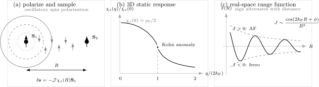
The RKKY response chain. (a) A local moment produces an oscillatory electron-spin polarization sampled by a second moment. (b) The normalized three-dimensional Lindhard response is continuous but nonanalytic at $q=2k_{\mathrm F}$. (c) Fourier transformation produces alternating ferro- and antiferromagnetic pair couplings with a $1/R^3$ envelope in an isotropic three-dimensional metal.

Three-Dimensional Range Function

For the continuum contact exchange and conventions above, the real-space spin susceptibility at $R>0$ is

$$\chi_s(R) = \frac{m} {32\pi^3\hbar^2R^4} \left[ \sin x - x\cos x \right], \qquad x=2k_{\mathrm F}R.$$

Therefore

$$J_{\mathrm{RKKY}}(R) = \frac{ \mathcal J^2mk_{\mathrm F}^4 }{ 2\pi^3\hbar^2 } \frac{ x\cos x-\sin x }{ x^4 }.$$

The prefactor assumes a point contact, a continuum field normalized by

$$\{ \psi_\sigma(\mathbf r), \psi_{\sigma'}^\dagger(\mathbf r') \} = \delta_{\sigma\sigma'} \delta(\mathbf r-\mathbf r'),$$

and a per-spin density of states. A lattice exchange, extended impurity orbital, or different spin normalization changes the amplitude and short-distance behavior.

At $k_{\mathrm F}R\gg1$,

$$J_{\mathrm{RKKY}}(R) \sim \frac{ \mathcal J^2mk_{\mathrm F} }{ 16\pi^3\hbar^2 } \frac{ \cos(2k_{\mathrm F}R) }{ R^3 }.$$

The oscillation period is

$$\Delta R_{\mathrm{period}} = \frac{\pi}{k_{\mathrm F}},$$

and successive asymptotic zero crossings are separated by

$$\Delta R_{\mathrm{zero}} = \frac{\pi}{2k_{\mathrm F}}.$$

The point-contact formula diverges as $R\to0$ and must not be trusted at atomic separations. Finite orbital extent, lattice-scale band structure, direct exchange, and superexchange then matter.

Fermi-Surface Origin

The asymptotic interaction is controlled by low-energy particle–hole excitations connecting points on the Fermi surface. For a smooth, convex Fermi surface, stationary-phase points have group velocities parallel or antiparallel to the separation $\mathbf R$. The relevant oscillation wavevectors are therefore calipers spanning the Fermi surface along $\mathbf R$.

For a generic isotropic metal in spatial dimension $d$,

$$J(R) \sim \frac{ \cos( 2k_{\mathrm F}R+\phi_d ) }{ R^d },$$

where the phase $\phi_d$ depends on convention and dimension.

Host	Generic long-distance behavior	Important qualification
One-dimensional metal	$R^{-1}$ oscillation	especially sensitive to interactions and boundaries
Two-dimensional parabolic metal	$R^{-2}$ oscillation	exact form uses Bessel functions
Three-dimensional parabolic metal	$R^{-3}$ oscillation	exact spherical range function given above
Nonspherical Fermi surface	direction-dependent periods and amplitudes	caliper vectors replace a single $2k_{\mathrm F}$
Nested or locally flat surface	enhanced response and potentially slower decay	curvature and matrix elements decide the power
Undoped Dirac system	nonmetallic power law	sublattice, valley, and symmetry structure can fix signs

The familiar rule “decay as $R^{-d}$” is not universal. It assumes an ordinary Fermi surface with nonzero local curvature and a pointlike coupling. Roth, Zeiger, and Kaplan showed that cylindrical or nearly parallel Fermi-surface regions can alter the decay and strengthen directionality.

Momentum-space ordering tendency

For local moments on a lattice, write

$$H_{\mathrm{RKKY}} = \frac{1}{2N} \sum_{\mathbf q} J(\mathbf q) \mathbf S_{\mathbf q} \cdot \mathbf S_{-\mathbf q}.$$

In the scalar weak-coupling limit,

$$J(\mathbf q) = - J_K^2 \chi_s(\mathbf q).$$

The classical exchange energy is minimized at the wavevector where $J(\mathbf q)$ is smallest, equivalently where $\chi_s(\mathbf q)$ is largest. A peak at $\mathbf q=\mathbf 0$ favors a uniform state; a peak at a finite $\mathbf Q$ favors antiferromagnetic, helical, or spin-density-modulated local-moment order depending on tensor structure and anisotropy.

The $2k_{\mathrm F}$ Kohn anomaly of the spherical three-dimensional gas is not generally its largest susceptibility. It controls the far-field oscillation even though $\chi_s(q)$ is largest at $q=0$ in that simple benchmark.

Material Corrections

Several bands and orbitals

In a crystal, $\chi_s^{ab}$ can carry band, orbital, sublattice, and basis-position indices. Intraband terms emphasize the Fermi surface; interband terms can remain important near avoided crossings or in spin–orbit-coupled systems. The exchange between moments on orbitals $\alpha$ and $\beta$ is more accurately written

$$J_{\alpha\beta}^{ab}(\mathbf R) = - J_{K,\alpha} \chi_{\alpha\beta}^{ab}(\mathbf R) J_{K,\beta}.$$

Orbital form factors can suppress a geometrically available spanning vector. A density-of-states-only estimate cannot predict this.

Spin–orbit coupling

Without spin-rotation symmetry, the response is a tensor and the pair Hamiltonian can be decomposed as

$$\begin{aligned} H_{ij} &= J_H \mathbf S_i\cdot\mathbf S_j + \mathbf D_{ij}\cdot ( \mathbf S_i\times\mathbf S_j ) \\ &\quad+ S_i^a \Gamma_{ij}^{ab} S_j^b. \end{aligned}$$

The antisymmetric susceptibility produces the Dzyaloshinskii–Moriya term, while its symmetric traceless part produces anisotropic exchange. Inversion and other bond symmetries can force some components to vanish. Exchange Interactions owns the full tensor and symmetry ledger.

Finite temperature

Thermal smearing rounds the Kohn anomaly. The corresponding thermal length is of order

$$\ell_T \sim \frac{\hbar v_{\mathrm F}} {k_{\mathrm B}T}.$$

For $R\ll\ell_T$, the zero-temperature range function is a good approximation. For $R\gtrsim\ell_T$, oscillations are thermally damped. Numerical factors involving $\pi$ depend on the dispersion and the precise asymptotic form.

Elastic disorder

In a weakly disordered metal, the disorder-averaged RKKY interaction is commonly damped on the mean-free-path scale:

$$\overline{ J(R) } \sim J_{\mathrm{clean}}(R) e^{-R/\ell}.$$

Sample-specific fluctuations need not vanish on exactly the same scale. Random impurity positions and oscillatory signs can therefore produce a broad distribution of couplings even when the spatial average is small.

Electron interactions

The most general weak local-moment coupling samples the interacting host susceptibility. Fermi-liquid parameters, paramagnons, vertex corrections, and collective modes can enhance or redirect the exchange:

$$J_{\mathrm{eff}}(\mathbf q) = - J_K^2 \chi_s^{\mathrm{host}}(\mathbf q).$$

Random Phase Approximation gives one controlled resummation only when its assumptions apply. Near an instability, truncating the moment–electron coupling at second order can fail even if an enhanced susceptibility looks tempting.

Gaps and nonmetallic hosts

A band gap, superconducting gap, pseudogap, or finite-size level spacing changes the long-distance response. In an ordinary gapped host, the interaction is generally cut off exponentially beyond a correlation or coherence length. Interband exchange in insulators is often classified as Bloembergen–Rowland exchange or another virtual-excitation mechanism rather than metallic RKKY. Naming the mediator and its low-energy spectrum is more useful than stretching the acronym.

From Pair Couplings to Magnetic Order

RKKY exchange can organize a lattice of local moments into ferro-, antiferro-, helical, or incommensurate order. The ordering vector is not obtained by inspecting one pair. It follows from the minimum eigenvalue of the full Fourier-space exchange matrix.

For a scalar Bravais-lattice model in the present sign convention, the Curie–Weiss temperature is

$$\Theta_{\mathrm{CW}} = - \frac{ S(S+1) }{ 3k_{\mathrm B} } \sum_j J_{ij}.$$

A negative $\Theta_{\mathrm{CW}}$ indicates a positive net exchange sum, but it need not equal the ordering temperature or reveal the ordering wavevector. Frustration, low dimension, anisotropy, disorder, and fluctuations can strongly separate those scales.

Mean-field ordering occurs schematically when

$$k_{\mathrm B}T_{\mathrm{MF}} = - \frac{ S(S+1) }{ 3 } \lambda_{\min},$$

where $\lambda_{\min}<0$ is the minimum eigenvalue of the exchange matrix in momentum and internal-index space. This estimate ignores critical fluctuations and does not establish the true transition temperature in low-dimensional or frustrated systems.

Dilute random moments

If local moments occupy random positions, the factor $2k_{\mathrm F}R_{ij}$ varies from pair to pair. The resulting mixed ferro- and antiferromagnetic bonds can generate frustration and glassy freezing. Oscillatory RKKY exchange is an important ingredient in canonical metallic spin glasses such as dilute CuMn or AuFe, but random signs alone do not prove a thermodynamic spin-glass phase. Aging, memory, nonlinear susceptibility, and frequency-dependent freezing must be tested.

Rare-earth metals and intermetallics

Localized $4f$ moments can couple through more extended $s$, $p$, and $d$ bands. Fermi-surface geometry then helps select long-period helices or commensurate order. Crystal-field anisotropy and several exchange channels must be included before comparing with neutron diffraction or spin-wave spectra.

Metallic multilayers and surfaces

Magnetic layers separated by a nonmagnetic metal can exhibit oscillatory interlayer exchange as spacer thickness changes. Surface-state-mediated interactions can be strongly directional and can be mapped by engineered adatom structures. These settings share the susceptibility and Fermi-surface logic of RKKY, although interfaces, quantum-well states, extended contacts, and multiple reflections modify the point-impurity range function.

Competition with Kondo Screening

The same antiferromagnetic local exchange can generate two qualitatively different tendencies:

• second-order RKKY coupling correlates distinct local moments;
• repeated local spin flips generate Kondo screening.

The schematic RKKY scale is algebraic,

$$k_{\mathrm B}T_{\mathrm{RKKY}} \sim C J_K^2 \rho_0,$$

whereas the single-impurity Kondo scale is nonanalytic in weak coupling. Kondo Lattices owns the scale comparison, the Doniach heuristic, and the collective phases beyond the impurity limit. Heavy Fermions owns the coherence-scale ledger and materials interpretation.

RKKY perturbation theory is most credible when the running local exchange remains weak at the energy and distance scales being probed. Once moments are substantially screened, treating a bare $J_K^2\chi_0$ pair coupling and independent single-impurity Kondo effects as additive is uncontrolled.

Experimental Inference

Pair spectroscopy

For two spin-$1/2$ moments with

$$H = J_{12} \mathbf S_1\cdot\mathbf S_2,$$

the singlet and triplet energies are

$$E_s = - \frac{3J_{12}}{4}, \qquad E_t = \frac{J_{12}}{4}.$$

Thus

$$E_t-E_s = J_{12}.$$

Inelastic tunnelling, neutron spectroscopy, or field-dependent level crossings can determine the sign and magnitude, provided single-ion anisotropy and other pair interactions are included.

Carrier-density tuning

Gate voltage, chemical doping, or pressure can change Fermi-surface dimensions. A sign reversal correlated with a change in a spanning vector is strong evidence for carrier-mediated oscillatory exchange. The comparison must use the measured or calculated multiband Fermi surface, not merely a spherical $k_{\mathrm F}$ inferred from total density.

Ordering and diffuse scattering

Neutron or resonant x-ray scattering measures the ordering wavevector and diffuse correlations above the transition. A successful RKKY model should reproduce:

1. the location and symmetry of response maxima;
2. the ordered structure;
3. spin-wave energies and intensities;
4. carrier-density and pressure trends;
5. the influence of disorder and crystal-field anisotropy.

Agreement with only a Curie–Weiss temperature is underdetermined.

Calculation workflow

A material calculation should report:

• the electronic structure and Fermi level;
• the local-moment orbitals and exchange vertices;
• the full static susceptibility matrix;
• Fourier and basis-position conventions;
• convergence in $\mathbf k$, $\mathbf q$, temperature, and broadening;
• whether interactions are included in the host response;
• the mapping from the response tensor to the spin Hamiltonian;
• validation against an independent observable.

Common Mistakes

Calling every long-range exchange RKKY

Metallic low-energy particle–hole response is the defining mediator. Superexchange, Bloembergen–Rowland exchange, double exchange, dipolar coupling, and quantum-well interlayer exchange can overlap in phenomenology but have different control parameters.

Inferring the sign from antiferromagnetic local exchange

$\mathcal J>0$ does not force $J_{\mathrm{RKKY}}>0$. The pair coupling is proportional to $\mathcal J^2$ and its sign comes from the spatial susceptibility.

Mixing response signs

A positive spin susceptibility defined with $H_h=-h s$ is not the same object as a negative density polarization defined with a positive potential-energy perturbation. Carry the source sign through the free-energy expansion.

Forgetting the pair-counting factor

The quadratic free energy contains $1/2\sum_{ij}$. The two cross terms combine into one $i<j$ pair; they do not leave an extra $1/2$.

Treating twice the Fermi wavevector as the ordering vector

$2k_{\mathrm F}$ controls a nonanalyticity and the far-field oscillation of the spherical gas. Magnetic order is selected by the minimum eigenvalue of the complete exchange matrix, equivalently by the relevant susceptibility maximum.

Using the spherical formula in a crystal

Nonspherical pockets, several bands, orbital matrix elements, basis positions, and spin–orbit coupling can alter periods, amplitudes, decay powers, and tensor structure.

Extrapolating to atomic separation

The continuum point-contact range function is a far-field result. At short distance, finite orbitals and other exchange mechanisms cannot be neglected.

Equating random bonds with a spin glass

Random oscillatory couplings create frustration, but spin-glass freezing requires thermodynamic and dynamical evidence.

Exercises

Exercise 1: Sign from the induced polarization

In the convention of this page, suppose $\chi_s(R)>0$ for two moments separated by $R$. What is the sign of $J_{\mathrm{RKKY}}(R)$, and which pair alignment is favored?

Solution

The pair coupling is

$$J_{\mathrm{RKKY}}(R) = - \mathcal J^2 \chi_s(R).$$

Since $\mathcal J^2>0$ and $\chi_s(R)>0$,

$$J_{\mathrm{RKKY}}(R) < 0.$$

With $H=J_{\mathrm{RKKY}}\mathbf S_1\cdot\mathbf S_2$, a negative coefficient favors parallel, ferromagnetic alignment. If a source uses $H=-I\mathbf S_1\cdot\mathbf S_2$, it will quote $I>0$ for the same physical result.

Exercise 2: Recover the pair-counting factor

For two moments, insert

$$h = h_1+h_2$$

into

$$\Delta F = - \frac12 h\chi h.$$

Show that the cross term is $-h_1\chi h_2$ rather than $-\frac12h_1\chi h_2$.

Solution

Expanding gives

$$\begin{aligned} \Delta F &= - \frac12 \left( h_1\chi h_1 + h_1\chi h_2 + h_2\chi h_1 + h_2\chi h_2 \right). \end{aligned}$$

Static reciprocity gives

$$h_2\chi h_1 = h_1\chi h_2.$$

Therefore the two cross terms combine:

$$\Delta F_{\mathrm{cross}} = - h_1\chi h_2.$$

The remaining diagonal terms are self-energy corrections for the individual moments.

Exercise 3: Far-field limit of the 3D range function

Starting from

$$J(R) = A \frac{ x\cos x-\sin x }{ x^4 }, \qquad x=2k_{\mathrm F}R,$$

find the leading large-$R$ behavior.

Solution

For $x\gg1$, the term $x\cos x$ is one power of $x$ larger than $\sin x$. Hence

$$\frac{ x\cos x-\sin x }{ x^4 } = \frac{\cos x}{x^3} + O(x^{-4}).$$

Since $x=2k_{\mathrm F}R$,

$$J(R) \sim \frac{A} {(2k_{\mathrm F})^3} \frac{ \cos(2k_{\mathrm F}R) }{ R^3 }.$$

The subleading sine term shifts finite-distance zero crossings but not the asymptotic decay power.

Exercise 4: Density-tuned sign reversal

Two moments have fixed separation $R=2.0\,\mathrm{nm}$. In the far-field approximation, what change $\Delta k_{\mathrm F}$ changes the phase $2k_{\mathrm F}R$ by $\pi$ and therefore reverses the cosine sign?

Solution

Require

$$2R\Delta k_{\mathrm F} = \pi.$$

Thus

$$\Delta k_{\mathrm F} = \frac{\pi}{2R} = \frac{\pi}{4.0\,\mathrm{nm}} \simeq 0.785\,\mathrm{nm^{-1}}.$$

The estimate assumes one spherical pocket and ignores any change in amplitude or orbital character. A multiband material can exhibit beating or no clean single sign reversal.

Exercise 5: Kohn anomaly versus ordering maximum

For the three-dimensional free-electron gas, $\chi_s(q)$ is largest at $q=0$ but has a derivative nonanalyticity at $q=2k_{\mathrm F}$. Which feature controls the ordering tendency in the scalar lattice approximation, and which controls the asymptotic real-space oscillation?

Solution

Because

$$J(q) = - J_K^2 \chi_s(q),$$

the exchange energy is minimized where $\chi_s(q)$ is largest. In the ideal spherical benchmark, that is $q=0$, so the scalar weak-coupling tendency is uniform.

The long-distance real-space oscillation is controlled by the nonanalytic structure at $q=2k_{\mathrm F}$. Fourier transforms retain algebraic tails from such nonanalyticities even when they are not global maxima. The two roles must not be conflated.

Exercise 6: Ordering wavevector from a susceptibility matrix

A material has two candidate wavevectors. The largest eigenvalue of its static spin susceptibility is $2.1\,\mathrm{eV^{-1}}$ at $\mathbf q=0$ and $3.4\,\mathrm{eV^{-1}}$ at $\mathbf Q$. Assume the same scalar $J_K$ couples to both channels. Which wavevector is selected at quadratic RKKY level?

Solution

The corresponding exchange eigenvalues are

$$\lambda_J(\mathbf q) = - J_K^2 \lambda_\chi(\mathbf q).$$

The larger susceptibility eigenvalue gives the more negative exchange eigenvalue. Therefore

$$\lambda_J(\mathbf Q) < \lambda_J(\mathbf 0),$$

and the quadratic RKKY energy selects $\mathbf Q$. The eigenvector at $\mathbf Q$, not the eigenvalue alone, determines the orbital, sublattice, and spin pattern. Nonlinear terms and fluctuations still decide the final phase and transition order.

Exercise 7: Thermal and disorder cutoffs

Take $v_{\mathrm F}=1.0\times10^6\,\mathrm{m\,s^{-1}}$, $T=50\,\mathrm K$, mean free path $\ell=20\,\mathrm{nm}$, and moment separation $R=100\,\mathrm{nm}$. Estimate $\ell_T=\hbar v_{\mathrm F}/(k_{\mathrm B}T)$ and the disorder-average factor $e^{-R/\ell}$. Which cutoff is more severe?

Solution

The thermal length is

$$\begin{aligned} \ell_T &= \frac{ (1.055\times10^{-34}) (1.0\times10^6) }{ (1.381\times10^{-23}) (50) } \mathrm m \\ &\simeq 1.53\times10^{-7}\,\mathrm m \\ &\simeq 153\,\mathrm{nm}. \end{aligned}$$

Since $R/\ell_T\simeq0.65$, thermal smearing is beginning to matter but has not placed the pair far beyond the thermal length.

The disorder factor is

$$e^{-R/\ell} = e^{-5} \simeq 6.74\times10^{-3}.$$

The disorder-averaged interaction is therefore much more strongly suppressed in this example. A particular sample can still have fluctuating couplings not represented by the simple average.

Connections

• Exchange Interactions compares microscopic exchange mechanisms and owns the general anisotropic tensor decomposition.
• Kondo Effect develops local screening, operational Kondo scales, impurity transport, and the screening cloud.
• Kondo Lattices develops Kondo–RKKY competition, lattice coherence, Fermi-volume counting, and Kondo-breakdown phase vocabulary.
• Heavy Fermions connects the local-moment competition to coherent heavy bands and cross-probe material evidence.
• Kondo Model Preview derives the local exchange flow whose weak-coupling square enters RKKY perturbation theory.
• Fermi Surface develops pockets, velocities, nesting, calipers, and experimental reconstruction.
• Susceptibilities fixes source signs, normalizations, static limits, matrices, and eigenchannels.
• Effective Hamiltonians in Many-Body Systems gives projection and perturbative control criteria.
• Random Phase Approximation treats interaction-renormalized response and matrix pole conditions.
• Ferromagnetism and Antiferromagnetism develop the ordered phases that susceptibility-mediated exchange can support.
• Glasses and Spin Glasses explains how random moment positions and sign-changing indirect exchange can generate frustrated collective freezing instead.
• Itinerant Magnetism distinguishes ordering of local moments through a carrier bath from magnetism formed by the band electrons themselves.
• Spin Waves and Magnons in Materials maps fitted exchange networks into dispersions, intensities, and stability tests.
• Long-Range Order supplies correlation and structure-factor diagnostics beyond mean field.
• Condensed-Matter Roadmap places indirect exchange after band structure, response, and local-moment formation.

References

1. M. A. Ruderman and C. Kittel, “Indirect Exchange Coupling of Nuclear Magnetic Moments by Conduction Electrons,” Physical Review 96, 99–102 (1954), doi:10.1103/PhysRev.96.99.
2. T. Kasuya, “A Theory of Metallic Ferro- and Antiferromagnetism on Zener’s Model,” Progress of Theoretical Physics 16, 45–57 (1956), doi:10.1143/PTP.16.45.
3. K. Yosida, “Magnetic Properties of Cu-Mn Alloys,” Physical Review 106, 893–898 (1957), doi:10.1103/PhysRev.106.893.
4. J. Lindhard, “On the Properties of a Gas of Charged Particles,” Kongelige Danske Videnskabernes Selskab, Matematisk-fysiske Meddelelser 28, no. 8 (1954), OSTI 4405425.
5. L. M. Roth, H. J. Zeiger, and T. A. Kaplan, “Generalization of the Ruderman–Kittel–Kasuya–Yosida Interaction for Nonspherical Fermi Surfaces,” Physical Review 149, 519–525 (1966), doi:10.1103/PhysRev.149.519.
6. B. Fischer and M. W. Klein, “Magnetic and Nonmagnetic Impurities in Two-Dimensional Metals,” Physical Review B 11, 2025–2029 (1975), doi:10.1103/PhysRevB.11.2025.
7. D. N. Aristov, “Indirect RKKY Interaction in Any Dimensionality,” Physical Review B 55, 8064–8066 (1997), doi:10.1103/PhysRevB.55.8064.
8. S. Doniach, “The Kondo Lattice and Weak Antiferromagnetism,” Physica B+C 91, 231–234 (1977), doi:10.1016/0378-4363(77)90190-5.
9. H. Imamura, P. Bruno, and Y. Utsumi, “Twisted Exchange Interaction between Localized Spins Embedded in a One- or Two-Dimensional Electron Gas with Rashba Spin–Orbit Coupling,” Physical Review B 69, 121303(R) (2004), doi:10.1103/PhysRevB.69.121303.
10. S. Saremi, “RKKY in Half-Filled Bipartite Lattices: Graphene as an Example,” Physical Review B 76, 184430 (2007), doi:10.1103/PhysRevB.76.184430.
11. S. S. P. Parkin, N. More, and K. P. Roche, “Oscillations in Exchange Coupling and Magnetoresistance in Metallic Superlattice Structures: Co/Ru, Co/Cr, and Fe/Cr,” Physical Review Letters 64, 2304–2307 (1990), doi:10.1103/PhysRevLett.64.2304.
12. L. Zhou et al., “Strength and Directionality of Surface Ruderman–Kittel–Kasuya–Yosida Interaction Mapped on the Atomic Scale,” Nature Physics 6, 187–191 (2010), doi:10.1038/nphys1514.
13. V. Cannella and J. A. Mydosh, “Magnetic Ordering in Gold-Iron Alloys,” Physical Review B 6, 4220–4237 (1972), doi:10.1103/PhysRevB.6.4220.
14. K. Binder and A. P. Young, “Spin Glasses: Experimental Facts, Theoretical Concepts, and Open Questions,” Reviews of Modern Physics 58, 801–976 (1986), doi:10.1103/RevModPhys.58.801.