Fermi Momentum and Fermi Energy

The Fermi momentum $p_{\mathrm F}=\hbar k_{\mathrm F}$ is the momentum at the boundary of the filled zero-temperature states of a uniform ideal Fermi gas. The Fermi energy is the one-particle energy at that boundary:

$$E_{\mathrm F} \equiv \epsilon(k_{\mathrm F}).$$

For a nonrelativistic particle of mass $m$,

$$E_{\mathrm F} = \frac{\hbar^2k_{\mathrm F}^2}{2m} = \frac{p_{\mathrm F}^2}{2m}.$$

These quantities are not independent thermodynamic parameters. Once the spatial dimension, number density, internal degeneracy, and dispersion are specified, state counting fixes $k_{\mathrm F}$ and hence every other Fermi scale.

The most common source of wrong factors is a silent change between:

• total density, summed over all internal components;
• density per spin or hyperfine component;
• spinless or fully polarized conventions;
• continuum momentum and crystal momentum;
• kinetic energy and total relativistic energy.

This page makes those conventions explicit and is the canonical dimension-by-dimension formula reference. The Ideal Fermi Gas page owns the full three-dimensional thermodynamic model, while Degenerate Fermi Gas owns the physical regime $T\ll T_{\mathrm F}$ and its applications.

Scope and notation

Unless stated otherwise, assume:

• a uniform continuum system in $d$ spatial dimensions;
• a large periodic box of $d$-dimensional measure $\mathcal V_d=L^d$;
• $N$ particles and total density $n=N/\mathcal V_d$;
• $g$ degenerate internal modes at every wave vector;
• an isotropic, monotonically increasing dispersion $\epsilon(k)$;
• zero temperature when defining the occupied Fermi region;
• one fermion at most in each complete one-particle mode.

The label internal mode may denote spin, hyperfine state, valley, flavor, or another independent quantum number. The factor $g$ may be used only when those modes are degenerate and have the same Fermi boundary.

This page writes the Fermi energy as $E_{\mathrm F}$. Many texts and neighboring pages write $\epsilon_{\mathrm F}$ for the same quantity. The notation does not imply a different physical definition:

$$E_{\mathrm F} = \epsilon_{\mathrm F} = \epsilon(k_{\mathrm F}).$$

At finite temperature, $E_{\mathrm F}$ remains the zero-temperature density scale. It is generally not equal to the temperature-dependent chemical potential $\mu(T)$.

Formula sheet

For a quadratic dispersion,

$$\epsilon(k) = \frac{\hbar^2k^2}{2m},$$

the standard formulas are:

Dimension	Total density	Fermi wave number
1D	$n=gk_{\mathrm F}/\pi$	$k_{\mathrm F}=\pi n/g$
2D	$n=gk_{\mathrm F}^2/(4\pi)$	$k_{\mathrm F}=\sqrt{4\pi n/g}$
3D	$n=gk_{\mathrm F}^3/(6\pi^2)$	$k_{\mathrm F}=(6\pi^2n/g)^{1/3}$

The corresponding Fermi energies are:

Dimension	Fermi energy
1D	$E_{\mathrm F}=\hbar^2\pi^2n^2/(2mg^2)$
2D	$E_{\mathrm F}=2\pi\hbar^2n/(mg)$
3D	$E_{\mathrm F}=\dfrac{\hbar^2}{2m}(6\pi^2n/g)^{2/3}$

For a balanced spin-$1/2$ gas, $g=2$ and $n$ is the total density:

$$\begin{array}{c|c} d & k_{\mathrm F} \\ \hline 1 & \pi n/2 \\ 2 & \sqrt{2\pi n} \\ 3 & (3\pi^2n)^{1/3} \end{array}$$

For a spinless or fully polarized gas, set $g=1$.

Geometric origin of the formulas

Periodic boundary conditions quantize each wave-vector component in steps of $2\pi/L$. One allowed $\mathbf k$ point per internal mode therefore occupies $d$-dimensional wave-vector volume

$$\left( \frac{2\pi}{L} \right)^d.$$

Equivalently, the number of wave-vector states per internal mode in an element $d^dk$ is

$$\frac{\mathcal V_d}{(2\pi)^d} \,d^dk.$$

Let $\Omega_d$ denote the volume of the unit ball in $d$ Euclidean dimensions:

$$\Omega_d = \frac{\pi^{d/2}} {\Gamma(d/2+1)}.$$

The ball of radius $k$ has volume $\Omega_d k^d$. Including $g$ internal modes, the integrated state count is

$$\mathcal N_d(k) = g \frac{\mathcal V_d}{(2\pi)^d} \Omega_d k^d.$$

At $T=0$, the ground state fills the $N$ lowest one-particle modes. For a monotone isotropic dispersion, this occupied region is the ball $|\mathbf k|\leq k_{\mathrm F}$, so

$$N = g \frac{\mathcal V_d}{(2\pi)^d} \Omega_d k_{\mathrm F}^d.$$

Dividing by $\mathcal V_d$ gives the master relation

$$n = g \frac{\Omega_d}{(2\pi)^d} k_{\mathrm F}^d.$$

Solving for the Fermi wave number,

$$k_{\mathrm F} = \left[ \frac{(2\pi)^d}{g\Omega_d} n \right]^{1/d}.$$

The numerical coefficients in 1D, 2D, and 3D are therefore geometric coefficients, not additional dynamical assumptions.

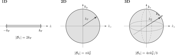
For an isotropic monotone dispersion, the zero-temperature occupied region is the $d$-ball $\mathcal B_d(k_{\mathrm F})$. Its geometric measure is $2k_{\mathrm F}$ in 1D, $\pi k_{\mathrm F}^2$ in 2D, and $4\pi k_{\mathrm F}^3/3$ in 3D. Multiplication by $g\mathcal V_d/(2\pi)^d$ converts that measure into a state count.

One dimension

In one dimension the occupied region is the interval

$$-k_{\mathrm F} \leq k \leq k_{\mathrm F}.$$

Its length is $2k_{\mathrm F}$. Since the density of allowed $k$ values per unit length and per internal mode is $1/(2\pi)$,

$$\frac{N}{L} = g \frac{1}{2\pi} (2k_{\mathrm F}).$$

Thus

$$n = \frac{gk_{\mathrm F}}{\pi}, \qquad k_{\mathrm F} = \frac{\pi n}{g}.$$

For the quadratic dispersion,

$$E_{\mathrm F} = \frac{\hbar^2\pi^2n^2} {2mg^2}.$$

The one-dimensional Fermi boundary consists of two points, $-k_{\mathrm F}$ and $+k_{\mathrm F}$. Calling those two points a Fermi surface is standard, even though each connected component has dimension zero.

For a balanced two-component gas, $g=2$ and

$$k_{\mathrm F} = \frac{\pi n}{2}.$$

If $n_\uparrow=n_\downarrow=n/2$, the same result can be written component by component as

$$k_{{\mathrm F},\sigma} = \pi n_\sigma.$$

These two equations agree. Mixing the total density $n$ with the per-component formula is what creates the familiar factor-of-two error.

Two dimensions

In two dimensions the occupied region is a disk of area $\pi k_{\mathrm F}^2$. State counting gives

$$n = g \frac{\pi k_{\mathrm F}^2} {(2\pi)^2} = \frac{gk_{\mathrm F}^2}{4\pi}.$$

Therefore

$$k_{\mathrm F} = \sqrt{ \frac{4\pi n}{g} }.$$

For a quadratic dispersion,

$$E_{\mathrm F} = \frac{2\pi\hbar^2n}{mg}.$$

For a balanced spin-$1/2$ gas,

$$k_{\mathrm F} = \sqrt{2\pi n}, \qquad E_{\mathrm F} = \frac{\pi\hbar^2n}{m}.$$

The two-dimensional Fermi boundary is a circle for an isotropic continuum dispersion. The energy density of states is constant for a quadratic band, but that fact follows from the energy–momentum relation rather than from the definition of $k_{\mathrm F}$ alone.

Three dimensions

In three dimensions the occupied region is a ball of volume $4\pi k_{\mathrm F}^3/3$. The density is

$$n = g \frac{1}{(2\pi)^3} \frac{4\pi k_{\mathrm F}^3}{3} = \frac{gk_{\mathrm F}^3}{6\pi^2}.$$

Hence

$$k_{\mathrm F} = \left( \frac{6\pi^2n}{g} \right)^{1/3}.$$

For a quadratic dispersion,

$$E_{\mathrm F} = \frac{\hbar^2}{2m} \left( \frac{6\pi^2n}{g} \right)^{2/3}.$$

For a balanced spin-$1/2$ gas,

$$k_{\mathrm F} = (3\pi^2n)^{1/3},$$

and

$$E_{\mathrm F} = \frac{\hbar^2}{2m} (3\pi^2n)^{2/3}.$$

This is the convention most often used for conduction electrons and balanced two-component atomic Fermi gases. The Ideal Fermi Gas page derives the associated three-dimensional density of states, energy, pressure, and finite-temperature thermodynamics.

Internal degeneracy conventions

The degeneracy factor counts independent one-particle modes at the same $\mathbf k$. It is part of the state count, not a correction applied after the count.

Spin degeneracy

If spin is conserved and all $2s+1$ spin projections are degenerate and equally populated, then

$$g_s = 2s+1.$$

Examples include:

• spinless fermions or a fully polarized sample: $g=1$;
• balanced spin-$1/2$ fermions: $g=2$;
• an idealized balanced spin-$3/2$ multiplet: $g=4$.

This formula does not say that every spin multiplet is physically populated. Zeeman splitting, spin–orbit coupling, preparation constraints, interactions, or selection rules may remove the degeneracy.

Several independent degeneracies

If spin, valley, and another internal label are all independent and exactly degenerate, their multiplicities multiply:

$$g = g_s g_v g_{\mathrm{other}}.$$

One must not multiply by a label that is already counted as a separate band or included explicitly in the sum over states.

Total density and component density

Suppose $g$ components are balanced, each with density $n_a$. Then

$$n = \sum_{a=1}^{g}n_a = g n_a.$$

The per-component state count contains no additional degeneracy factor:

$$n_a = \frac{\Omega_d}{(2\pi)^d} k_{\mathrm F}^d.$$

Substituting $n_a=n/g$ recovers the total-density formula.

Imbalanced components

If components have unequal densities, there is generally no single common Fermi wave number. Each component has

$$k_{{\mathrm F},a} = \left[ \frac{(2\pi)^d}{\Omega_d} n_a \right]^{1/d}.$$

For two spin components in three dimensions,

$$k_{{\mathrm F},\uparrow} = (6\pi^2n_\uparrow)^{1/3}, \qquad k_{{\mathrm F},\downarrow} = (6\pi^2n_\downarrow)^{1/3}.$$

Writing one $g=2$ formula for an imbalanced gas hides the two distinct Fermi surfaces.

Fixed-density polarization effect

At fixed total density,

$$k_{\mathrm F} \propto g^{-1/d},$$

and, for a quadratic dispersion,

$$E_{\mathrm F} \propto g^{-2/d}.$$

Reducing the number of available internal components forces particles to occupy a larger region of momentum space. In three dimensions, fully polarizing a previously balanced spin-$1/2$ ideal gas changes the scales by

$$\frac{k_{\mathrm F}^{(g=1)}} {k_{\mathrm F}^{(g=2)}} = 2^{1/3},$$

and

$$\frac{E_{\mathrm F}^{(g=1)}} {E_{\mathrm F}^{(g=2)}} = 2^{2/3}.$$

Derived Fermi scales

Once $k_{\mathrm F}$ is known, several useful scales follow.

Fermi momentum

Wave number and momentum differ by $\hbar$:

$$p_{\mathrm F} = \hbar k_{\mathrm F}.$$

Thus $k_{\mathrm F}$ has units of inverse length, while $p_{\mathrm F}$ has units of momentum. The phrase Fermi momentum is often used informally for either quantity; a careful formula should display which one is meant.

Fermi velocity

For a general isotropic dispersion, the group velocity at the Fermi boundary is

$$v_{\mathrm F} = \frac{1}{\hbar} \left. \frac{d\epsilon}{dk} \right|_{k=k_{\mathrm F}}.$$

For a quadratic dispersion,

$$v_{\mathrm F} = \frac{\hbar k_{\mathrm F}}{m} = \sqrt{ \frac{2E_{\mathrm F}}{m} }.$$

Fermi temperature

The Fermi temperature is the energy scale expressed in kelvin:

$$T_{\mathrm F} \equiv \frac{E_{\mathrm F}}{k_{\mathrm B}}.$$

It is not the temperature of the zero-temperature gas. It defines the reduced temperature

$$\theta = \frac{T}{T_{\mathrm F}},$$

which distinguishes the degenerate regime $\theta\ll1$ from the classical regime $\theta\gg1$ under the appropriate density conditions.

Fermi wavelength and inverse Fermi scale

The de Broglie wavelength associated with $p_{\mathrm F}$ is

$$\lambda_{\mathrm F} = \frac{h}{p_{\mathrm F}} = \frac{2\pi}{k_{\mathrm F}}.$$

Many-body estimates also use the shorter length $k_{\mathrm F}^{-1}$. These differ by $2\pi$ and should not be interchanged silently.

Fermi time

A natural microscopic time is

$$t_{\mathrm F} = \frac{\hbar}{E_{\mathrm F}}.$$

For a quadratic dispersion,

$$t_{\mathrm F} = \frac{2m}{\hbar k_{\mathrm F}^2}.$$

This is a scale, not automatically a collision time or equilibration time.

Density scaling by dimension

For fixed $g$,

$$k_{\mathrm F} \propto n^{1/d}.$$

With a quadratic dispersion,

$$E_{\mathrm F} \propto n^{2/d}, \qquad v_{\mathrm F} \propto n^{1/d}.$$

Therefore:

Dimension	$k_{\mathrm F}$ scaling	$E_{\mathrm F}$ scaling
1D	$n$	$n^2$
2D	$n^{1/2}$	$n$
3D	$n^{1/3}$	$n^{2/3}$

The stronger density dependence in lower dimension reflects how rapidly the occupied interval or disk must expand when particles are added.

Inverse formulas

If the nonrelativistic Fermi energy is known, then

$$k_{\mathrm F} = \frac{\sqrt{2mE_{\mathrm F}}}{\hbar}.$$

The corresponding density in $d$ dimensions is

$$n = g \frac{\Omega_d}{(2\pi)^d} \left( \frac{2mE_{\mathrm F}}{\hbar^2} \right)^{d/2}.$$

Explicitly,

$$\begin{aligned} n_{1\mathrm D} &= \frac{g}{\pi} \frac{\sqrt{2mE_{\mathrm F}}}{\hbar}, \\ n_{2\mathrm D} &= \frac{gmE_{\mathrm F}} {2\pi\hbar^2}, \\ n_{3\mathrm D} &= \frac{g}{6\pi^2} \left( \frac{2mE_{\mathrm F}}{\hbar^2} \right)^{3/2}. \end{aligned}$$

The densities have different dimensions: inverse length in 1D, inverse area in 2D, and inverse volume in 3D.

Density-of-states checks

The integrated number of states below energy $E$ for a quadratic dispersion is

$$\frac{\mathcal N_d(E)}{\mathcal V_d} = g \frac{\Omega_d}{(2\pi)^d} \left( \frac{2mE}{\hbar^2} \right)^{d/2}.$$

Differentiation gives the density of states per $d$-dimensional measure:

$$\rho_d(E) = \frac{1}{\mathcal V_d} \frac{d\mathcal N_d}{dE}.$$

At the Fermi energy,

$$\rho_d(E_{\mathrm F}) = \frac{d}{2} \frac{n}{E_{\mathrm F}}.$$

This identity is a fast consistency check. It uses a density of states that includes the same internal factor $g$ as the density $n$.

The energy dependence is

$$\rho_d(E) \propto E^{d/2-1}.$$

Thus the free-particle density of states diverges as $E^{-1/2}$ in 1D, is constant in 2D, and grows as $E^{1/2}$ in 3D. The canonical discussion of density-of-states normalization is Density of States: First Encounter.

Zero-temperature consistency identities

For a quadratic dispersion, integrating all occupied energies gives

$$\frac{U_0}{N} = \frac{d}{d+2} E_{\mathrm F}.$$

Scale invariance of the nonrelativistic kinetic energy gives

$$P_0 = \frac{2}{d} \frac{U_0}{\mathcal V_d} = \frac{2}{d+2} nE_{\mathrm F}.$$

In one dimension, $P_0$ is a force; in two dimensions, it is force per length; in three dimensions, it is the usual force per area. These identities are useful checks, but the full equation-of-state derivation belongs to the Ideal Fermi Gas page.

Worked example: a three-dimensional electron density

Consider nonrelativistic electrons with total density

$$n = 8.5\times10^{28}\ \mathrm{m}^{-3}$$

and spin degeneracy $g=2$. Then

$$k_{\mathrm F} = (3\pi^2n)^{1/3} \approx 1.36\times10^{10}\ \mathrm{m}^{-1}.$$

The momentum scale is

$$p_{\mathrm F} = \hbar k_{\mathrm F} \approx 1.43\times10^{-24}\ \mathrm{kg\,m\,s^{-1}}.$$

Using the electron mass,

$$E_{\mathrm F} = \frac{\hbar^2k_{\mathrm F}^2}{2m_e} \approx 7.0\ \mathrm{eV}.$$

Consequently,

$$v_{\mathrm F} \approx 1.6\times10^6\ \mathrm{m\,s^{-1}},$$

and

$$T_{\mathrm F} \approx 8.1\times10^4\ \mathrm K.$$

An ordinary laboratory temperature can therefore be much smaller than $T_{\mathrm F}$ even when it is hundreds of kelvin. This is why conduction electrons are often strongly degenerate. A real metal may require band-dependent effective masses and a nonspherical Fermi surface, so the numerical calculation is an ideal free-electron estimate rather than a complete material model.

Worked example: a two-dimensional electron gas

Take a two-dimensional spin-degenerate gas with sheet density

$$n_{2\mathrm D} = 1.0\times10^{15}\ \mathrm{m}^{-2},$$

$g=2$, and effective mass $m^*=0.067m_e$. The Fermi wave number is

$$k_{\mathrm F} = \sqrt{2\pi n_{2\mathrm D}} \approx 7.93\times10^7\ \mathrm{m}^{-1}.$$

The quadratic-band Fermi energy is

$$E_{\mathrm F} = \frac{\pi\hbar^2n_{2\mathrm D}}{m^*} \approx 3.6\ \mathrm{meV}.$$

Equivalently,

$$T_{\mathrm F} \approx 41\ \mathrm K.$$

The use of $m^*$ rather than the bare electron mass is part of the model specification. Valley degeneracy, spin splitting, or nonparabolicity would modify the count or the dispersion.

Worked example: changing spin polarization

Consider a three-dimensional gas at fixed total density $n$. In a balanced two-component state,

$$k_{\mathrm F}^{\mathrm{bal}} = (3\pi^2n)^{1/3}.$$

In a fully polarized state,

$$k_{\mathrm F}^{\mathrm{pol}} = (6\pi^2n)^{1/3}.$$

Therefore

$$k_{\mathrm F}^{\mathrm{pol}} = 2^{1/3} k_{\mathrm F}^{\mathrm{bal}},$$

and

$$E_{\mathrm F}^{\mathrm{pol}} = 2^{2/3} E_{\mathrm F}^{\mathrm{bal}}.$$

The change is a direct consequence of Pauli filling: fewer internal modes are available at each $\mathbf k$, so the occupied momentum-space region must grow.

What survives for another dispersion

The state-counting relation for $k_{\mathrm F}$ depends on the occupied $k$-space volume, not on the detailed energy dispersion. For any monotone isotropic band, the same density relation holds:

$$n = g \frac{\Omega_d}{(2\pi)^d} k_{\mathrm F}^d.$$

Only the map from $k_{\mathrm F}$ to energy and velocity changes:

$$E_{\mathrm F} = \epsilon(k_{\mathrm F}),$$

and

$$v_{\mathrm F} = \frac{1}{\hbar} \epsilon'(k_{\mathrm F}).$$

For a power-law dispersion

$$\epsilon(k) = A k^s,$$

one obtains

$$E_{\mathrm F} \propto n^{s/d},$$

and

$$\rho_d(E_{\mathrm F}) = \frac{d}{s} \frac{n}{E_{\mathrm F}}.$$

The familiar factor $d/2$ is the special case $s=2$.

Relativistic convention

Relativistic state counting gives the same $k_{\mathrm F}$ for a specified density and degeneracy. What changes is the energy relation. With

$$p_{\mathrm F} = \hbar k_{\mathrm F},$$

the total one-particle energy at the Fermi boundary is

$$\mathcal E_{\mathrm F} = \sqrt{ p_{\mathrm F}^2c^2 + m^2c^4 }.$$

If Fermi energy means kinetic energy measured from the rest energy, then

$$E_{\mathrm F}^{\mathrm{kin}} = \sqrt{ p_{\mathrm F}^2c^2 + m^2c^4 } - mc^2.$$

At zero temperature, a relativistic chemical potential that includes rest energy is

$$\mu_0 = \mathcal E_{\mathrm F},$$

whereas a convention that subtracts rest energy gives

$$\mu_0^{\mathrm{kin}} = E_{\mathrm F}^{\mathrm{kin}}.$$

Both conventions are legitimate; mixing them in one calculation is not. The nonrelativistic approximation requires

$$p_{\mathrm F} \ll mc.$$

Bands, lattices, and anisotropy

The scalar $k_{\mathrm F}$ is exact for a spherical Fermi boundary. In a crystal band, the occupied region is determined by

$$E_n(\mathbf k) \leq \mu_0,$$

inside the Brillouin zone. The boundary can be warped, disconnected, open across a zone boundary, or split among bands. Then one should speak of:

• the Fermi surface $E_n(\mathbf k)=\mu_0$;
• direction-dependent Fermi wave vectors;
• extremal radii or orbit areas;
• an effective spherical $k_{\mathrm F}$ only when explicitly defined.

For an anisotropic quadratic band,

$$\epsilon(\mathbf k) = \frac{\hbar^2}{2} \left( \frac{k_x^2}{m_x} + \frac{k_y^2}{m_y} + \frac{k_z^2}{m_z} \right),$$

constant-energy surfaces are ellipsoids. Replacing all masses by one $m$ without stating an approximation loses the geometry that fixes the state count.

Fermi Surface develops the general many-body concept and low-energy excitations near nonspherical boundaries. The future Quantum Matter treatment will own detailed Bloch-band topology and material-specific surfaces.

Traps and inhomogeneous gases

A finite trap does not have translational invariance, so momentum states are not labeled by a uniform continuum density. Exact state counting uses trap eigenlevels.

In a slowly varying potential, a local-density approximation may define

$$n(\mathbf r) = g \frac{\Omega_d}{(2\pi)^d} k_{\mathrm F}(\mathbf r)^d,$$

with a local Fermi energy

$$E_{\mathrm F}(\mathbf r) = \frac{\hbar^2k_{\mathrm F}(\mathbf r)^2}{2m}.$$

These are local scales. They need not equal the global Fermi energy defined by the highest occupied trap level. Quantum Gases in Traps owns the trap conventions and local-density application.

Finite systems and shell filling

In a finite box, allowed momenta are discrete. The continuum formula replaces a lattice-point count by a geometric volume, so it becomes accurate when many modes are occupied and boundary corrections are small.

For a finite noninteracting system, several quantities may be called the Fermi energy:

• the highest occupied one-particle energy;
• the lowest unoccupied one-particle energy;
• the midpoint between them;
• an addition or removal chemical potential;
• the continuum estimate from the mean density.

They coincide in the thermodynamic limit under regular conditions but can differ by a shell spacing in a small system. A partially filled degenerate shell also makes the zero-temperature boundary less sharp than the continuum picture suggests.

Practical calculation workflow

Use the following sequence.

1. Identify the geometry. Decide whether the system is uniform, trapped, or periodic on a lattice.
2. Specify the dimension. A line density, sheet density, and volume density have different units.
3. List internal components. Determine whether spin, valley, flavor, or band labels are explicit or absorbed into $g$.
4. Choose total or component density. Write the choice next to the symbol $n$.
5. Count the occupied wave-vector region. For a spherical continuum gas, use the $d$-ball formula.
6. Map wave number to energy. Insert the actual dispersion, bare mass, effective mass, or relativistic relation.
7. State the energy zero. Say whether rest energy or a band minimum has been subtracted.
8. Check the regime. Test finite-size, temperature, anisotropy, interaction, and relativistic assumptions.

Canonical boundaries

This page owns:

• the general $d$-dimensional continuum state count;
• explicit 1D, 2D, and 3D formulas for $n$, $k_{\mathrm F}$, and $E_{\mathrm F}$;
• total-density and per-component conventions;
• internal-degeneracy and polarization factors;
• derived scales $p_{\mathrm F}$, $v_{\mathrm F}$, $T_{\mathrm F}$, $\lambda_{\mathrm F}$, and $t_{\mathrm F}$;
• reference checks involving the density of states;
• warnings for finite, trapped, anisotropic, lattice, and relativistic systems.

Other pages own:

• the complete uniform three-dimensional ideal-gas thermodynamics: Ideal Fermi Gas;
• the low-temperature regime, Pauli blocking, and applications: Degenerate Fermi Gas;
• the occupation function at finite temperature: Fermi–Dirac Statistics;
• density-of-states normalization and broader uses: Density of States: First Encounter;
• generic Fermi-surface geometry and low-energy kinematics: Fermi Surface;
• low-temperature asymptotic integration: Sommerfeld Expansion;
• interacting quasiparticles and renormalized Fermi-liquid parameters: later many-body and quantum-matter pages.

Common mistakes

Calling wave number momentum

$k_{\mathrm F}$ has units of inverse length. The momentum is $p_{\mathrm F}=\hbar k_{\mathrm F}$.

Using the spin-1/2 formula for a spinless gas

The common three-dimensional result $(3\pi^2n)^{1/3}$ assumes $g=2$ and total density. A spinless gas instead has $(6\pi^2n)^{1/3}$.

Double-counting spin

If $n_\sigma$ is a per-spin density, do not also multiply its state count by $g=2$. If $n$ is total density, include all occupied components exactly once.

Assigning one Fermi wave number to an imbalanced gas

Unequal component densities imply unequal $k_{{\mathrm F},a}$ unless another constraint changes the simple model.

Equating Fermi energy with chemical potential at every temperature

For the ideal gas, $\mu(0)=E_{\mathrm F}$ under the same energy convention. At finite temperature, $\mu(T)$ generally differs from $E_{\mathrm F}$.

Using a three-dimensional density in a two-dimensional formula

A sheet density has units $\mathrm m^{-2}$, while a volume density has units $\mathrm m^{-3}$. A quasi-two-dimensional layer also requires a clear convention for its effective thickness.

Using the bare mass in an effective band

For a parabolic semiconductor band, use the stated effective mass. For a nonparabolic or anisotropic band, one scalar effective mass may be inadequate.

Treating a lattice Fermi surface as a sphere

Crystal momentum lives in a Brillouin zone and the band dispersion sets the boundary shape. A spherical $k_{\mathrm F}$ is then an approximation or an effective definition.

Forgetting the energy zero

Relativistic total energy, kinetic energy, and band energy measured from a minimum differ by additive constants. State the convention before comparing $E_{\mathrm F}$ with $\mu$.

Using continuum formulas for a few particles

Small systems exhibit shell effects and boundary-condition dependence. Count discrete levels when the level spacing is not negligible.

Exercises

Derive the master count

A uniform ideal Fermi gas occupies a $d$-dimensional periodic box of measure $\mathcal V_d$. Show that a filled ball of radius $k_{\mathrm F}$ contains

$$N = g \frac{\mathcal V_d\Omega_d}{(2\pi)^d} k_{\mathrm F}^d$$

states. State where each factor comes from.

Solution

Periodic boundary conditions give a spacing $2\pi/L$ in each wave-vector direction. One allowed point therefore occupies wave-vector volume

$$\left( \frac{2\pi}{L} \right)^d,$$

so the number of points per $d^dk$ is

$$\frac{L^d}{(2\pi)^d} = \frac{\mathcal V_d}{(2\pi)^d}.$$

The occupied $d$-ball has volume $\Omega_dk_{\mathrm F}^d$. Multiplying by the point density and by $g$ independent internal modes gives

$$N = g \frac{\mathcal V_d}{(2\pi)^d} \Omega_dk_{\mathrm F}^d.$$

The factors represent internal multiplicity, real-space measure, reciprocal-space normalization, and occupied reciprocal-space volume, respectively.

Recover all three dimensional formulas

Use

$$\Omega_1=2, \qquad \Omega_2=\pi, \qquad \Omega_3=\frac{4\pi}{3}$$

to derive $n(k_{\mathrm F})$ in 1D, 2D, and 3D.

Solution

Insert each unit-ball volume into

$$n = g \frac{\Omega_d}{(2\pi)^d} k_{\mathrm F}^d.$$

For $d=1$,

$$n = g \frac{2}{2\pi} k_{\mathrm F} = \frac{gk_{\mathrm F}}{\pi}.$$

For $d=2$,

$$n = g \frac{\pi}{(2\pi)^2} k_{\mathrm F}^2 = \frac{gk_{\mathrm F}^2}{4\pi}.$$

For $d=3$,

$$n = g \frac{4\pi/3}{(2\pi)^3} k_{\mathrm F}^3 = \frac{gk_{\mathrm F}^3}{6\pi^2}.$$

Translate between total and component density

A balanced two-component gas in two dimensions has total sheet density $n$. Compute $k_{\mathrm F}$ first from the total-density formula with $g=2$, then from the density $n_\sigma=n/2$ of one component. Verify agreement.

Solution

Using total density and $g=2$,

$$k_{\mathrm F} = \sqrt{ \frac{4\pi n}{2} } = \sqrt{2\pi n}.$$

For one component, no extra degeneracy factor is included:

$$n_\sigma = \frac{k_{\mathrm F}^2}{4\pi}.$$

Since $n_\sigma=n/2$,

$$k_{\mathrm F} = \sqrt{4\pi n_\sigma} = \sqrt{2\pi n}.$$

The two routes agree because they count the same modes with different bookkeeping.

Compare balanced and polarized gases

At fixed total density in dimension $d$, compare a balanced gas with degeneracy $g$ to a fully polarized gas with degeneracy $1$. Find the ratios of Fermi wave numbers and nonrelativistic Fermi energies.

Solution

At fixed density,

$$k_{\mathrm F} \propto g^{-1/d}.$$

Therefore

$$\frac{k_{\mathrm F}^{(1)}} {k_{\mathrm F}^{(g)}} = g^{1/d}.$$

For a quadratic dispersion, $E_{\mathrm F}\propto k_{\mathrm F}^2$, so

$$\frac{E_{\mathrm F}^{(1)}} {E_{\mathrm F}^{(g)}} = g^{2/d}.$$

The polarized gas fills farther in momentum space because fewer internal modes are available at each wave vector.

Derive the density-of-states check

Starting from $\mathcal N_d(E)/\mathcal V_d\propto E^{d/2}$ for a quadratic dispersion, show that

$$\rho_d(E_{\mathrm F}) = \frac{d}{2} \frac{n}{E_{\mathrm F}}.$$

Solution

Write

$$\frac{\mathcal N_d(E)}{\mathcal V_d} = C E^{d/2},$$

where $C$ contains the mass, degeneracy, and geometric factors. Differentiation gives

$$\rho_d(E) = \frac{d}{2} C E^{d/2-1}.$$

At $E=E_{\mathrm F}$,

$$n = C E_{\mathrm F}^{d/2}.$$

Eliminating $C$ yields

$$\rho_d(E_{\mathrm F}) = \frac{d}{2} \frac{n}{E_{\mathrm F}}.$$

Obtain the mean ground-state energy

Use $\rho_d(E)\propto E^{d/2-1}$ to prove

$$\frac{U_0}{N} = \frac{d}{d+2} E_{\mathrm F}.$$

Check the results in 1D, 2D, and 3D.

Solution

The particle number and energy are proportional to

$$N \propto \int_0^{E_{\mathrm F}} E^{d/2-1}\,dE = \frac{2}{d} E_{\mathrm F}^{d/2},$$

and

$$U_0 \propto \int_0^{E_{\mathrm F}} E^{d/2}\,dE = \frac{2}{d+2} E_{\mathrm F}^{d/2+1}.$$

Taking the ratio gives

$$\frac{U_0}{N} = \frac{d}{d+2} E_{\mathrm F}.$$

Thus

$$\frac{U_0}{N} = \begin{cases} E_{\mathrm F}/3, & d=1,\\ E_{\mathrm F}/2, & d=2,\\ 3E_{\mathrm F}/5, & d=3. \end{cases}$$

Check the two-dimensional numerical example

For $n_{2\mathrm D}=1.0\times10^{15}\ \mathrm{m}^{-2}$, $g=2$, and $m^*=0.067m_e$, calculate $k_{\mathrm F}$, $E_{\mathrm F}$, and $T_{\mathrm F}$. Use

$$\hbar = 1.0546\times10^{-34}\ \mathrm{J\,s},$$ $$m_e = 9.109\times10^{-31}\ \mathrm{kg},$$

and

$$k_{\mathrm B} = 1.3806\times10^{-23}\ \mathrm{J\,K^{-1}}.$$

Solution

The wave number is

$$\begin{aligned} k_{\mathrm F} &= \sqrt{2\pi n_{2\mathrm D}} \\ &\approx 7.93\times10^7\ \mathrm{m}^{-1}. \end{aligned}$$

The effective mass is

$$m^* \approx 6.10\times10^{-32}\ \mathrm{kg}.$$

Therefore

$$\begin{aligned} E_{\mathrm F} &= \frac{\hbar^2k_{\mathrm F}^2}{2m^*} \\ &\approx 5.72\times10^{-22}\ \mathrm J \\ &\approx 3.57\ \mathrm{meV}. \end{aligned}$$

Finally,

$$T_{\mathrm F} = \frac{E_{\mathrm F}}{k_{\mathrm B}} \approx 41.4\ \mathrm K.$$

Separate relativistic energy conventions

Show that the relativistic kinetic Fermi energy approaches $p_{\mathrm F}^2/(2m)$ when $p_{\mathrm F}\ll mc$, and approaches $p_{\mathrm F}c$ when $p_{\mathrm F}\gg mc$.

Solution

The kinetic Fermi energy is

$$E_{\mathrm F}^{\mathrm{kin}} = mc^2 \left[ \sqrt{ 1+ \left( \frac{p_{\mathrm F}}{mc} \right)^2 } -1 \right].$$

For $x=p_{\mathrm F}/(mc)\ll1$,

$$\sqrt{1+x^2} = 1+ \frac{x^2}{2} + O(x^4),$$

so

$$E_{\mathrm F}^{\mathrm{kin}} = \frac{p_{\mathrm F}^2}{2m} + O\!\left( \frac{p_{\mathrm F}^4}{m^3c^2} \right).$$

For $x\gg1$,

$$\sqrt{1+x^2} = x+ O(x^{-1}),$$

and therefore

$$E_{\mathrm F}^{\mathrm{kin}} = p_{\mathrm F}c - mc^2 + O\!\left( \frac{m^2c^3}{p_{\mathrm F}} \right).$$

The leading density-dependent term is $p_{\mathrm F}c$. The subtractive rest-energy constant remains because the kinetic-energy convention measures from $mc^2$.

Cross-links

• Fermi Gas Formula Sheet
• Ideal Fermi Gas
• Degenerate Fermi Gas
• Fermi Surface
• Fermi–Dirac Statistics
• Occupation Numbers
• Chemical Potential
• Thermodynamic Limit
• Density of States: First Encounter
• Plane Waves and Delta Normalization
• Pauli Exclusion Principle
• Ideal Fermi Gas Model Card
• Density of States Formula Card

References

• R. K. Pathria and P. D. Beale, Statistical Mechanics, 3rd ed., Elsevier (2011) — continuum state counting and ideal quantum gases.
• K. Huang, Statistical Mechanics, 2nd ed., Wiley (1987) — ideal Fermi-gas thermodynamics and dimensional state counting.
• M. Kardar, Statistical Physics of Particles, Cambridge University Press (2007) — phase-space counting and quantum statistics.
• A. L. Fetter and J. D. Walecka, Quantum Theory of Many-Particle Systems, Dover (2003) — Fermi momentum, density of states, and many-body conventions.
• N. W. Ashcroft and N. D. Mermin, Solid State Physics, Holt, Rinehart and Winston (1976) — free-electron and band-theory Fermi scales.
• G. F. Giuliani and G. Vignale, Quantum Theory of the Electron Liquid, Cambridge University Press (2005) — electron-gas conventions in two and three dimensions.
• S. Giorgini, L. P. Pitaevskii, and S. Stringari, “Theory of ultracold atomic Fermi gases,” Reviews of Modern Physics 80, 1215–1274 (2008) — balanced and imbalanced atomic-gas conventions.
• X.-W. Guan, M. T. Batchelor, and C. Lee, “Fermi gases in one dimension: From Bethe ansatz to experiments,” Reviews of Modern Physics 85, 1633–1691 (2013) — one-dimensional Fermi scales and component conventions.