Maxwell–Boltzmann Limit

The Maxwell–Boltzmann limit is the dilute regime in which the equilibrium occupations of ideal bosonic and fermionic modes agree at leading order:

$$\overline n_i \simeq z e^{-\beta\epsilon_i} = e^{-\beta(\epsilon_i-\mu)}.$$

Here

$$z = e^{\beta\mu}, \qquad \beta = \frac{1}{k_{\mathrm B}T},$$

and $i$ labels a complete one-particle mode. The approximation is controlled mode by mode by

$$y_i \equiv z e^{-\beta\epsilon_i} \ll 1.$$

For a uniform nonrelativistic gas in $d$ dimensions, this becomes the familiar phase-space-density condition

$$\mathcal D \equiv \frac{n\lambda_T^d}{g} \ll 1,$$

where

$$\lambda_T = \sqrt{ \frac{2\pi\hbar^2}{m k_{\mathrm B}T} }$$

is the thermal de Broglie wavelength and $g$ counts equally populated internal modes.

This limit does not make identical quantum particles fundamentally distinguishable. It makes exchange corrections small for the observables and accuracy under consideration. Bosons remain in symmetric states, fermions remain in antisymmetric states, and the factor $1/N!$ remains essential in the canonical partition function.

Purpose and Canonical Boundary

This page is a calculation guide for using the Maxwell–Boltzmann approximation. It owns:

• the distinction between a Boltzmann weight, a normalized one-particle probability, and a mean mode occupation;
• the normalization ladder from $q_1$ to $z$, density, and thermodynamics;
• canonical multinomial and grand-canonical Poisson descriptions;
• Maxwell momentum and speed distributions;
• dilute density profiles in external potentials and traps;
• practical accuracy checks and application workflows.

The full emergence from Bose–Einstein and Fermi–Dirac statistics, including fugacity expansions, exchange cycles, leading quantum virial corrections, dimensional generalizations, and interaction caveats, belongs to Classical Limit of Quantum Statistics. This page quotes those results when they are needed but does not duplicate their derivations.

The Quantum Statistics Overview compares the three regimes. The separate Bose–Einstein and Fermi–Dirac pages own the exact ideal-mode laws.

Assumptions

The standard formulas below combine several approximations. State them separately.

1. Thermal equilibrium: a temperature $T$ describes the relevant degrees of freedom.
2. Dilute quantum statistics: every appreciably occupied complete mode has $y_i\ll1$.
3. Ideal or controlled interactions: interactions are absent or incorporated through an additional approximation.
4. Nonrelativistic translation: $\epsilon_{\mathbf p}=p^2/(2m)$ when the thermal-wavelength formulas are used.
5. Semiclassical state counting: sums over translational levels may be replaced by phase-space integrals when explicitly done below.
6. Specified ensemble: total particle number is fixed in canonical formulas and fluctuates in grand-canonical formulas.

These assumptions are independent. A gas can be Maxwell–Boltzmann dilute while retaining a discrete quantum spectrum, or it can have an almost continuous spectrum while being quantum degenerate.

Four Objects That Must Not Be Confused

Many errors come from writing the same exponential for conceptually different quantities.

Boltzmann weight

For a one-particle energy $\epsilon_i$, the unnormalized equilibrium weight is

$$w_i = e^{-\beta\epsilon_i}.$$

This expression contains no normalization and no particle number.

One-particle partition function

The one-particle partition function is

$$q_1 = \sum_i e^{-\beta\epsilon_i}.$$

The sum runs over complete one-particle modes, including internal labels. Some texts call this quantity $Z_1$; here $q_1$ keeps it distinct from the $N$-particle canonical partition function.

Normalized one-particle probability

For one particle in a canonical thermal state,

$$p_i = \frac{e^{-\beta\epsilon_i}}{q_1}.$$

It satisfies

$$\sum_i p_i = 1.$$

This probability answers: “Given one particle, in which mode is it found?”

Mean occupation of a mode

For $N$ ideal particles in the Maxwell–Boltzmann regime,

$$\overline n_i = N p_i.$$

Equivalently, in grand-canonical notation,

$$\overline n_i = z e^{-\beta\epsilon_i}.$$

Consistency requires

$$N = z q_1,$$

so

$$z = \frac{N}{q_1}.$$

The probability $p_i$ is normalized to one; the occupation $\overline n_i$ is normalized to $N$. Confusing them usually loses either a factor of $N$ or the partition function.

The Short Quantum-Statistics Argument

Use

$$\eta = \begin{cases} +1, & \text{bosons},\\ -1, & \text{fermions}. \end{cases}$$

The exact ideal-mode occupation is

$$f_{\eta}(\epsilon_i) = \frac{y_i}{1-\eta y_i}.$$

For $y_i\ll1$,

$$f_{\eta}(\epsilon_i) = y_i + \eta y_i^2 + O(y_i^3).$$

Retaining only the first term gives

$$f_{\mathrm{MB}}(\epsilon_i) = y_i = z e^{-\beta\epsilon_i}.$$

The Bose/Fermi distinction first appears at order $y_i^2$. The canonical derivation, including the relation to permutation cycles and the equation of state, is given on Classical Limit of Quantum Statistics.

Uniform Nonrelativistic Gas

Consider a large $d$-dimensional box of volume $V$ with dispersion

$$\epsilon_{\mathbf p} = \frac{p^2}{2m}.$$

Let $g$ count internal states with the same translational energy. In the semiclassical approximation,

$$q_1 = gV \int \frac{d^d p}{(2\pi\hbar)^d} e^{-\beta p^2/(2m)}.$$

The Gaussian integral is

$$\int d^d p\, e^{-\beta p^2/(2m)} = \left( \frac{2\pi m}{\beta} \right)^{d/2}.$$

Therefore

$$q_1 = \frac{gV}{\lambda_T^d}.$$

Using $N=zq_1$ gives

$$z = \frac{N\lambda_T^d}{gV} = \frac{n\lambda_T^d}{g} = \mathcal D.$$

Thus, at leading Maxwell–Boltzmann order for a uniform gas,

$$z \simeq \mathcal D.$$

The equality receives Bose or Fermi corrections beyond leading order. It also assumes the simple continuum spectrum and a common internal population.

Canonical Counting and the Gibbs Factor

For $N$ identical particles in the dilute ideal-gas regime,

$$Z_N^{\mathrm{MB}} = \frac{q_1^N}{N!}.$$

The factor $1/N!$ removes overcounting of permutations of identical particles. It does not arise because the particles have become permanently labeled. Dropping it would describe $N$ distinguishable species with one member each, not one gas of identical particles.

Occupation-count probability

Let $n_i$ be the number of particles assigned to mode $i$, with

$$\sum_i n_i = N.$$

At Maxwell–Boltzmann order, the canonical probability of an occupation pattern is multinomial:

$$\Pr(\{n_i\}\mid N) = N! \prod_i \frac{p_i^{n_i}}{n_i!}.$$

Its moments are

$$\langle n_i\rangle = N p_i,$$ $$\operatorname{Var}(n_i) = N p_i(1-p_i),$$

and, for $i\neq j$,

$$\operatorname{Cov}(n_i,n_j) = -N p_i p_j.$$

The negative covariance comes from fixing the total number. It is an ensemble constraint, not a fermionic exchange effect.

If the one-particle state space is very large and every $p_i$ is small, then

$$\operatorname{Var}(n_i) \simeq \langle n_i\rangle.$$

That local Poisson approximation coexists with exact canonical anticorrelations among modes.

Grand-Canonical Counting

Insert $Z_N^{\mathrm{MB}}=q_1^N/N!$ into the grand partition function:

$$\begin{aligned} \Xi_{\mathrm{MB}} &= \sum_{N=0}^{\infty} z^N Z_N^{\mathrm{MB}} \\ &= \sum_{N=0}^{\infty} \frac{(zq_1)^N}{N!} \\ &= e^{zq_1}. \end{aligned}$$

The mean total number is

$$\overline N = z \frac{\partial\ln\Xi}{\partial z} = zq_1.$$

The total-number distribution is Poissonian:

$$\Pr(N) = e^{-\overline N} \frac{\overline N^N}{N!}.$$

Consequently,

$$\operatorname{Var}(N) = \overline N.$$

Each mode is also independently Poissonian at Maxwell–Boltzmann order:

$$\Pr_i(n) = e^{-y_i} \frac{y_i^n}{n!}, \qquad \overline n_i = \operatorname{Var}(n_i) = y_i.$$

This exact mode independence belongs to the grand-canonical Maxwell–Boltzmann model. Fixed-$N$ conditioning converts the independent Poisson variables into the multinomial law above.

Momentum Distribution

For a uniform nonrelativistic gas, the normalized one-particle momentum density is

$$\mathcal P(\mathbf p) = \left( \frac{\beta}{2\pi m} \right)^{d/2} e^{-\beta p^2/(2m)}.$$

It is normalized with respect to $d^d p$:

$$\int d^d p\, \mathcal P(\mathbf p) = 1.$$

Each Cartesian component is Gaussian:

$$\mathcal P(p_a) = \sqrt{ \frac{\beta}{2\pi m} } e^{-\beta p_a^2/(2m)}.$$

Therefore

$$\langle p_a\rangle = 0, \qquad \langle p_a^2\rangle = m k_{\mathrm B}T.$$

The mean translational kinetic energy per particle is

$$\left\langle \frac{p^2}{2m} \right\rangle = \frac{d}{2} k_{\mathrm B}T.$$

This is the equipartition result for $d$ quadratic momentum components. It follows here from the Maxwell distribution, not from an assumption about particle collisions.

The Three-Dimensional Speed Distribution

In three dimensions, transform from velocity components to the speed $v=|\mathbf v|$. The angular measure contributes $4\pi v^2$, giving

$$\mathcal P_v(v) = 4\pi \left( \frac{m}{2\pi k_{\mathrm B}T} \right)^{3/2} v^2 e^{-mv^2/(2k_{\mathrm B}T)}, \qquad v\geq0.$$

The factor $v^2$ is geometric. Although the vector distribution is largest at $\mathbf v=0$, the speed distribution vanishes at $v=0$ because a spherical shell of zero radius has zero phase-space volume.

Define the most probable speed

$$v_{\mathrm{mp}} = \sqrt{ \frac{2k_{\mathrm B}T}{m} }.$$

With

$$x = \frac{v}{v_{\mathrm{mp}}},$$

the normalized dimensionless density is

$$\mathcal P_x(x) = \frac{4}{\sqrt\pi} x^2 e^{-x^2}.$$

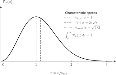
The dimensionless three-dimensional speed density $\mathcal P_x(x)=4x^2e^{-x^2}/\sqrt\pi$ for $x=v/v_{\mathrm{mp}}$. The most probable, mean, and root-mean-square speeds are different summaries of the same skewed distribution.

The characteristic speeds are

$$v_{\mathrm{mp}} = \sqrt{ \frac{2k_{\mathrm B}T}{m} },$$ $$\langle v\rangle = \sqrt{ \frac{8k_{\mathrm B}T}{\pi m} },$$ $$v_{\mathrm{rms}} = \sqrt{\langle v^2\rangle} = \sqrt{ \frac{3k_{\mathrm B}T}{m} }.$$

They satisfy

$$v_{\mathrm{mp}} < \langle v\rangle < v_{\mathrm{rms}}.$$

More generally,

$$\langle v^r\rangle = \left( \frac{2k_{\mathrm B}T}{m} \right)^{r/2} \frac{ \Gamma\!\left( \frac{r+3}{2} \right) }{ \Gamma\!\left( \frac{3}{2} \right) }.$$

External Potentials

Let the semiclassical one-particle energy be

$$\epsilon(\mathbf r,\mathbf p) = \frac{p^2}{2m} + V(\mathbf r).$$

The Maxwell–Boltzmann phase-space occupation is

$$f_{\mathrm{MB}}(\mathbf r,\mathbf p) = z e^{-\beta[p^2/(2m)+V(\mathbf r)]}.$$

Integrating over momentum gives the local number density

$$\begin{aligned} n(\mathbf r) &= g \int \frac{d^d p}{(2\pi\hbar)^d} f_{\mathrm{MB}}(\mathbf r,\mathbf p) \\ &= \frac{g z}{\lambda_T^d} e^{-\beta V(\mathbf r)}. \end{aligned}$$

Thus the spatial profile obeys

$$\frac{n(\mathbf r)}{n(\mathbf r_0)} = e^{-\beta[V(\mathbf r)-V(\mathbf r_0)]}.$$

This ratio is independent of $z$, $g$, and the momentum normalization.

Local degeneracy criterion

Define

$$\mathcal D(\mathbf r) = \frac{n(\mathbf r)\lambda_T^d}{g}.$$

At Maxwell–Boltzmann order,

$$\mathcal D(\mathbf r) = z e^{-\beta V(\mathbf r)}.$$

The approximation must hold where the gas is densest:

$$\max_{\mathbf r} \mathcal D(\mathbf r) \ll 1.$$

Dilute outer wings can be classical even when the center of a trapped gas is quantum degenerate.

Barometric profile

For a uniform gravitational potential $V(h)=mgh$,

$$n(h) = n(0) e^{-mgh/(k_{\mathrm B}T)}.$$

The scale height is

$$H = \frac{k_{\mathrm B}T}{mg}.$$

This result assumes isothermal equilibrium and neglects interactions and variations in the gravitational field.

Harmonic trap

For

$$V(\mathbf r) = \frac{m}{2} \sum_{a=1}^{d} \omega_a^2 x_a^2,$$

the density is Gaussian:

$$n(\mathbf r) = n(0) \exp\!\left[ -\frac{\beta m}{2} \sum_{a=1}^{d} \omega_a^2 x_a^2 \right].$$

The semiclassical one-particle partition function is

$$q_1^{\mathrm{trap}} = g \prod_{a=1}^{d} \frac{1}{\beta\hbar\omega_a}.$$

Hence

$$z = \frac{N}{q_1^{\mathrm{trap}}} = \frac{N}{g} \prod_{a=1}^{d} (\beta\hbar\omega_a).$$

The center is Maxwell–Boltzmann dilute when $z\ll1$. The condition depends on the trap frequencies and total particle number, not on a box density.

Thermodynamics of the Uniform Ideal Gas

For

$$q_1 = \frac{gV}{\lambda_T^d}, \qquad Z_N = \frac{q_1^N}{N!},$$

Stirling’s approximation gives

$$\ln N! = N\ln N-N+O(\ln N).$$

The Helmholtz free energy is

$$F = -k_{\mathrm B}T\ln Z_N \simeq N k_{\mathrm B}T \left[ \ln\!\left( \frac{n\lambda_T^d}{g} \right) -1 \right].$$

Equation of state

Using

$$P = - \left( \frac{\partial F}{\partial V} \right)_{T,N},$$

one obtains

$$PV = N k_{\mathrm B}T.$$

This equation requires both dilute statistics and ideal interactions. Maxwell–Boltzmann occupations alone do not guarantee the ideal-gas law if collisions produce a significant virial correction.

Internal energy and heat capacity

Because $\lambda_T^{-d}\propto T^{d/2}$,

$$U = - \frac{\partial\ln Z_N}{\partial\beta} = \frac{d}{2} N k_{\mathrm B}T.$$

Therefore

$$C_V = \left( \frac{\partial U}{\partial T} \right)_{V,N} = \frac{d}{2} N k_{\mathrm B}.$$

Internal excitations, rotations, vibrations, or relativistic dispersion add their own temperature-dependent contributions.

Chemical potential

The leading chemical potential is

$$\mu = \left( \frac{\partial F}{\partial N} \right)_{T,V} = k_{\mathrm B}T \ln\!\left( \frac{n\lambda_T^d}{g} \right).$$

Equivalently,

$$\beta\mu = \ln\mathcal D, \qquad z = \mathcal D.$$

The dilute condition $\mathcal D\ll1$ therefore corresponds to

$$\beta\mu \ll 0$$

when the translational ground-state energy is chosen as zero. Under an energy-zero shift, both $\epsilon_i$ and $\mu$ shift, while $\epsilon_i-\mu$ remains invariant.

Entropy

From

$$S = - \left( \frac{\partial F}{\partial T} \right)_{V,N},$$

the translational entropy is

$$\frac{S}{N k_{\mathrm B}} = \frac{d}{2} + 1 - \ln\!\left( \frac{n\lambda_T^d}{g} \right).$$

In three dimensions,

$$\frac{S}{N k_{\mathrm B}} = \frac{5}{2} - \ln\!\left( \frac{n\lambda_T^3}{g} \right),$$

the Sackur–Tetrode form with an internal degeneracy factor. The absolute normalization depends on quantum state counting through $h$ or $\hbar$ even though the resulting gas is in a classical statistical regime.

Internal Structure

A constant factor $g$ is adequate only when $g$ internal modes are degenerate and equally available. For internal energies $E_a$, define

$$q_{\mathrm{int}}(T) = \sum_a g_a e^{-\beta E_a}.$$

For a uniform three-dimensional nonrelativistic gas,

$$q_1 = \frac{V}{\lambda_T^3} q_{\mathrm{int}}(T).$$

Then

$$z = \frac{n\lambda_T^3}{q_{\mathrm{int}}(T)}.$$

If $q_{\mathrm{int}}$ depends on temperature, internal states contribute to energy and heat capacity:

$$U_{\mathrm{int}} = -N \frac{\partial\ln q_{\mathrm{int}}}{\partial\beta}.$$

One should not replace a resolved spin splitting, rotational ladder, or electronic spectrum by a constant degeneracy unless the relevant limits justify it.

Mixtures

For species $s$ with particle number $N_s$, mass $m_s$, internal partition factor $q_{\mathrm{int},s}$, and thermal wavelength $\lambda_{T,s}$,

$$Z_{\{N_s\}} = \prod_s \frac{q_{1,s}^{N_s}}{N_s!}.$$

Each species has its own dilute parameter

$$\mathcal D_s = \frac{n_s\lambda_{T,s}^d}{g_s}$$

when a constant degeneracy $g_s$ is appropriate. A mixture is safely Maxwell–Boltzmann only if every component that is being approximated satisfies its own criterion.

The factorial is species-specific. There is no division by

$$\left( \sum_s N_s \right)!$$

because particles of different species are distinguishable by physical quantum numbers.

Chemical reactions impose relations among species chemical potentials. In that setting, independently assigning every $\mu_s$ is generally inconsistent with equilibrium stoichiometry.

Quantitative Accuracy

“Small occupation” should be converted into an error estimate.

One-mode occupation error

The exact ideal occupation satisfies

$$\frac{f_{\eta}}{y} = \frac{1}{1-\eta y}.$$

The relative correction to the Maxwell–Boltzmann value is

$$\frac{f_{\eta}-y}{y} = \frac{\eta y}{1-\eta y}.$$

For $y\ll1$,

$$\left| \frac{f_{\eta}-y}{y} \right| \simeq y.$$

Thus a one-percent target for a particular mode requires roughly $y\lesssim10^{-2}$, with the precise bound depending on whether the correction is Bose or Fermi.

Pressure error

For a uniform ideal gas in $d$ dimensions, the leading exchange correction at fixed density is

$$\frac{P}{n k_{\mathrm B}T} = 1 - \eta \frac{\mathcal D}{2^{d/2+1}} + O(\mathcal D^2).$$

In three dimensions,

$$\frac{1}{2^{5/2}} \simeq 0.177.$$

The pressure can therefore be more accurate than the most occupied low-energy mode because it averages over the spectrum. Conversely, a low-energy-sensitive observable may fail before the bulk equation of state does.

Observable-specific criterion

There is no universal scalar error for “the Maxwell–Boltzmann approximation.” For an observable

$$A = \sum_i a_i n_i,$$

compare

$$\langle A\rangle_{\eta} = \sum_i a_i f_{\eta}(\epsilon_i)$$

with

$$\langle A\rangle_{\mathrm{MB}} = \sum_i a_i y_i.$$

The weights $a_i$ determine which energies matter. A condition based on a bulk average can miss a failure localized in the lowest mode or near a detector threshold.

Statistical Diluteness Is Not the Same as Classical Motion

Three approximations are often bundled together but need separate checks.

Maxwell–Boltzmann exchange limit

This requires small mode activities:

$$y_i \ll 1.$$

It suppresses exchange corrections.

Semiclassical state counting

Replacing a level sum by

$$\sum_i \longrightarrow g \int \frac{d^d r\,d^d p}{(2\pi\hbar)^d}$$

requires level spacings and spatial variations to be unresolved on thermal scales. For a harmonic trap, a common condition is

$$k_{\mathrm B}T \gg \hbar\omega_a.$$

This can fail even when $z\ll1$.

Classical trajectories

A phase-space distribution does not automatically justify assigning sharply localized trajectories. Wave-packet spreading, tunneling, interference, and discrete internal dynamics can remain important. Decoherence and dynamical length scales require separate analysis.

Two useful counterexamples

1. A cold trap with mean occupancy $\overline N\ll1$ can have $z\ll1$, while its discrete oscillator spectrum and zero-point structure remain quantum.
2. A dense gas in a very large box can have nearly continuous one-particle levels while $n\lambda_T^d/g\gtrsim1$, so Bose or Fermi exchange remains essential.

The word “classical” should always be accompanied by the approximation actually being made.

Interactions and Nonideality

The condition

$$n\lambda_T^d/g \ll 1$$

controls exchange statistics, not the strength of the interaction potential. A gas may be nondegenerate yet have appreciable interaction corrections.

For a dilute interacting gas, the equation of state has a virial form

$$\frac{P}{k_{\mathrm B}T} = n + B_2(T)n^2 + B_3(T)n^3 + \cdots.$$

The second virial coefficient can contain both exchange and interaction contributions:

$$B_2(T) = B_2^{\mathrm{exchange}}(T) + B_2^{\mathrm{interaction}}(T).$$

Maxwell–Boltzmann occupation statistics is not enough for the ideal equation of state if

$$n|B_2(T)| \not\ll 1.$$

At low energy, scattering lengths, bound states, resonances, and channel structure can dominate the interaction part. The Beth–Uhlenbeck relation provides the systematic two-body quantum correction through scattering phase shifts and bound states.

Finite and Discrete Spectra

For a finite set of levels, the most reliable criterion is the mode condition itself:

$$\max_i \left[ z e^{-\beta\epsilon_i} \right] \ll 1.$$

If the ground energy is $\epsilon_0$, this is

$$z e^{-\beta\epsilon_0} \ll 1.$$

The thermal-wavelength criterion may be unavailable or misleading for:

• a few-level system;
• a lattice with a finite band;
• a strongly anisotropic trap;
• a finite box with thermally resolved level spacings;
• particles with a nonquadratic dispersion.

In these cases, retain the exact one-particle partition sum

$$q_1 = \sum_i e^{-\beta\epsilon_i}$$

and use

$$z = \frac{N}{q_1}$$

at Maxwell–Boltzmann order. A phase-space integral is optional, not part of the definition.

Relativistic and Massless Particles

The Maxwell–Boltzmann form

$$\overline n_i \simeq z e^{-\beta\epsilon_i}$$

does not require a nonrelativistic dispersion. What changes is the one-particle state count:

$$q_1 = gV \int \frac{d^d p}{(2\pi\hbar)^d} e^{-\beta\epsilon(\mathbf p)}.$$

For relativistic particles,

$$\epsilon(\mathbf p) = \sqrt{p^2c^2+m^2c^4}.$$

The nonrelativistic thermal wavelength $\lambda_T\propto T^{-1/2}$ must then be replaced by the appropriate relativistic scale and integral.

For photons in ordinary equilibrium, $\mu=0$ and $z=1$. Low-frequency modes have

$$y = e^{-\beta\hbar\omega} \to 1$$

as $\omega\to0$, so a global Maxwell–Boltzmann approximation to blackbody radiation fails. The Wien tail, where $\beta\hbar\omega\gg1$, is Maxwell–Boltzmann-like even though the full spectrum is Bose–Einstein.

Worked Examples

Two-level internal structure

Suppose a particle has a nondegenerate internal ground state of energy zero and an excited manifold of degeneracy $r$ at energy $\Delta$. Then

$$q_{\mathrm{int}} = 1 + r e^{-\beta\Delta}.$$

The excited-state probability for one particle is

$$p_{\mathrm e} = \frac{r e^{-\beta\Delta}}{ 1+r e^{-\beta\Delta} }.$$

For a uniform three-dimensional gas,

$$z = \frac{n\lambda_T^3}{ 1+r e^{-\beta\Delta} }.$$

At $k_{\mathrm B}T\ll\Delta$, the excited manifold freezes out. At $k_{\mathrm B}T\gg\Delta$, it contributes an effective degeneracy $1+r$.

Dilute particles in a harmonic trap

For an isotropic three-dimensional trap with frequency $\omega$,

$$q_1 = g \left( \frac{k_{\mathrm B}T}{\hbar\omega} \right)^3$$

in the semiclassical regime. Hence

$$z = \frac{N}{g} \left( \frac{\hbar\omega}{k_{\mathrm B}T} \right)^3.$$

The Maxwell–Boltzmann center criterion is

$$\frac{N}{g} \left( \frac{\hbar\omega}{k_{\mathrm B}T} \right)^3 \ll 1.$$

This displays how cooling, increasing particle number, or tightening the trap drives the center toward quantum degeneracy.

A resolved finite spectrum

Take one-particle levels $\epsilon_0=0$, $\epsilon_1=\Delta$, and $\epsilon_2=3\Delta$, with no degeneracy. Then

$$q_1 = 1 + e^{-\beta\Delta} + e^{-3\beta\Delta}.$$

For fixed mean number $N$ at Maxwell–Boltzmann order,

$$z = \frac{N}{ 1+e^{-\beta\Delta}+e^{-3\beta\Delta} }.$$

The approximation requires $z\ll1$ because the ground-state activity is the largest. No thermal wavelength is needed, and the level discreteness is retained exactly.

Practical Workflow

1. Define complete modes. Include spin, polarization, band, valley, trap, and species labels.
2. Choose the energy zero. Keep $\epsilon_i-\mu$ invariant when shifting it.
3. Compute $q_1$. Use an exact sum or a justified phase-space integral.
4. Determine $z$. At Maxwell–Boltzmann order, use $z=N/q_1$ or the reservoir value $e^{\beta\mu}$.
5. Check the largest activity. Verify $\max_i z e^{-\beta\epsilon_i}\ll1$.
6. Check interactions separately. Estimate virial, scattering, or mean-field corrections.
7. Normalize the requested observable. Distinguish one-particle probabilities from mode occupations and total densities.
8. Estimate the error. Compare the first neglected Bose/Fermi term for the observable of interest.
9. Test limiting cases. Check normalization, dimensions, $T\to\infty$, low-density behavior, and any resolved spectral gaps.

Common Mistakes

Equating a Boltzmann factor with a probability

The factor $e^{-\beta\epsilon_i}$ is not normalized. Divide by $q_1$ for a one-particle probability or multiply by $z$ for a mean mode occupation.

Setting the fugacity to one

For a conserved dilute gas,

$$z = e^{\beta\mu} \ll 1.$$

Setting $z=1$ changes the density and generally violates the dilute criterion. The special case $\mu=0$ applies to particular nonconserved quasiparticles, not to every classical gas.

Dropping the Gibbs factor

Exchange corrections can be negligible while $1/N!$ remains necessary. The factor prevents the Gibbs paradox and gives an extensive entropy for one species.

Omitting internal degeneracy from the phase-space criterion

The per-mode parameter is

$$\mathcal D = \frac{n\lambda_T^3}{g}$$

for equally populated internal states. Resolved or polarized populations require species- or state-specific checks.

Calling every exponential distribution Maxwell–Boltzmann statistics

Canonical quantum systems of any exchange type use Boltzmann weights over many-body energy eigenstates. Maxwell–Boltzmann particle statistics is the dilute occupation regime with its associated counting.

Confusing speed with a velocity component

A velocity component is Gaussian and can be negative. Speed is nonnegative and has the $v^2$ shell factor in three dimensions.

Assuming ideality from nondegeneracy

Small exchange corrections do not imply weak interactions. Check the virial or scattering scale independently.

Replacing every discrete sum by an integral

The Maxwell–Boltzmann limit is an occupation approximation. A phase-space integral requires a separate semiclassical condition.

Using a bulk criterion for a nonuniform center

Trapped gases become degenerate first where the local density is largest. Check $\max_{\mathbf r}\mathcal D(\mathbf r)$, not only a volume-averaged density.

Exercises

Probability versus occupation

One-particle levels have energies $0$, $\Delta$, and $2\Delta$, with degeneracies $1$, $2$, and $1$. Find the normalized probability for each energy level and the mean occupation of each level for $N$ Maxwell–Boltzmann particles.

Solution

The one-particle partition function is

$$q_1 = 1 + 2e^{-\beta\Delta} + e^{-2\beta\Delta}.$$

The probabilities of the energy levels are

$$p_0 = \frac{1}{q_1},$$ $$p_1 = \frac{2e^{-\beta\Delta}}{q_1},$$ $$p_2 = \frac{e^{-2\beta\Delta}}{q_1}.$$

They sum to one. The mean level occupations are

$$\overline N_j = N p_j.$$

Within the twofold-degenerate middle level, each complete mode has mean occupation

$$\frac{N e^{-\beta\Delta}}{q_1}.$$

Degeneracy multiplies the level probability because it counts distinct modes.

Recover the thermal wavelength

Evaluate the three-dimensional momentum integral and show that

$$q_1 = \frac{gV}{\lambda_T^3}.$$

Solution

Start from

$$q_1 = gV \int \frac{d^3p}{(2\pi\hbar)^3} e^{-\beta p^2/(2m)}.$$

The Cartesian Gaussian factorizes:

$$\int d^3p\, e^{-\beta p^2/(2m)} = \left( \int_{-\infty}^{\infty} dp_x\, e^{-\beta p_x^2/(2m)} \right)^3.$$

Using

$$\int_{-\infty}^{\infty} dx\, e^{-a x^2} = \sqrt{ \frac{\pi}{a} },$$

one gets

$$\int d^3p\, e^{-\beta p^2/(2m)} = \left( \frac{2\pi m}{\beta} \right)^{3/2}.$$

Therefore

$$q_1 = gV \left( \frac{m}{2\pi\beta\hbar^2} \right)^{3/2}.$$

Since

$$\lambda_T = \sqrt{ \frac{2\pi\beta\hbar^2}{m} },$$

this becomes

$$q_1 = \frac{gV}{\lambda_T^3}.$$

Maxwell speed moments

Starting from

$$\mathcal P_x(x) = \frac{4}{\sqrt\pi} x^2e^{-x^2},$$

find the most probable value of $x$, the mean $\langle x\rangle$, and $\sqrt{\langle x^2\rangle}$.

Solution

Differentiate:

$$\frac{d}{dx} \left( x^2e^{-x^2} \right) = 2x(1-x^2)e^{-x^2}.$$

The nonzero maximum is at

$$x_{\mathrm{mp}} = 1.$$

For the mean,

$$\begin{aligned} \langle x\rangle &= \frac{4}{\sqrt\pi} \int_0^{\infty} x^3e^{-x^2} dx \\ &= \frac{2}{\sqrt\pi}. \end{aligned}$$

For the second moment,

$$\begin{aligned} \langle x^2\rangle &= \frac{4}{\sqrt\pi} \int_0^{\infty} x^4e^{-x^2} dx \\ &= \frac{3}{2}. \end{aligned}$$

Hence

$$\sqrt{\langle x^2\rangle} = \sqrt{ \frac{3}{2} }.$$

Multiplying by $v_{\mathrm{mp}}$ reproduces the three characteristic speeds in the text.

Poisson to multinomial conditioning

Suppose independent mode counts $n_i$ are Poisson variables with means $y_i$. Show that the total $N=\sum_i n_i$ is Poisson with mean $Y=\sum_i y_i$, and that conditioning on $N$ gives a multinomial distribution with probabilities $p_i=y_i/Y$.

Solution

The joint probability is

$$\Pr(\{n_i\}) = e^{-Y} \prod_i \frac{y_i^{n_i}}{n_i!}.$$

The generating function of the total number is

$$\begin{aligned} G(t) &= \prod_i e^{y_i(t-1)} \\ &= e^{Y(t-1)}, \end{aligned}$$

which is the generating function of a Poisson variable with mean $Y$:

$$\Pr(N) = e^{-Y} \frac{Y^N}{N!}.$$

Divide the joint probability by $\Pr(N)$ for configurations satisfying $\sum_i n_i=N$:

$$\begin{aligned} \Pr(\{n_i\}\mid N) &= N! \prod_i \frac{(y_i/Y)^{n_i}}{n_i!} \\ &= N! \prod_i \frac{p_i^{n_i}}{n_i!}. \end{aligned}$$

This is the multinomial law.

Harmonic-trap criterion

For $N$ particles in a three-dimensional anisotropic harmonic trap, derive the Maxwell–Boltzmann criterion in terms of $T$, $N$, $g$, and $\omega_x\omega_y\omega_z$.

Solution

The semiclassical one-particle partition function is

$$q_1 = g \frac{1}{ (\beta\hbar)^3 \omega_x\omega_y\omega_z }.$$

At Maxwell–Boltzmann order,

$$z = \frac{N}{q_1} = \frac{N}{g} (\beta\hbar)^3 \omega_x\omega_y\omega_z.$$

The largest local activity occurs at the trap center. Therefore the dilute criterion is

$$\frac{N}{g} \frac{ \hbar^3\omega_x\omega_y\omega_z }{ (k_{\mathrm B}T)^3 } \ll 1.$$

The semiclassical trap approximation additionally requires $k_{\mathrm B}T\gg\hbar\omega_a$ for each direction. These are separate conditions.

A one-percent error target

For a fermionic mode, find a sufficient upper bound on $y$ such that the relative difference between the exact Fermi occupation and the Maxwell–Boltzmann value is below one percent.

Solution

For fermions,

$$f_{\mathrm F} = \frac{y}{1+y}.$$

Relative to the Maxwell–Boltzmann value $y$,

$$\left| \frac{f_{\mathrm F}-y}{y} \right| = \frac{y}{1+y}.$$

Require

$$\frac{y}{1+y} < 0.01.$$

Solving gives

$$y < \frac{0.01}{0.99} \simeq 0.0101.$$

The simple rule $y\lesssim10^{-2}$ is therefore sufficient at this accuracy.

Internal freeze-out

A particle has a ground state of degeneracy $g_0$ and an excited state of degeneracy $g_1$ at energy $\Delta$. Find the internal contribution to the mean energy per particle and its low- and high-temperature limits.

Solution

The internal partition function is

$$q_{\mathrm{int}} = g_0 + g_1e^{-\beta\Delta}.$$

The excited-state probability is

$$p_1 = \frac{ g_1e^{-\beta\Delta} }{ g_0+g_1e^{-\beta\Delta} }.$$

Therefore

$$\frac{U_{\mathrm{int}}}{N} = \Delta p_1.$$

For $k_{\mathrm B}T\ll\Delta$,

$$\frac{U_{\mathrm{int}}}{N} \simeq \Delta \frac{g_1}{g_0} e^{-\beta\Delta},$$

which is exponentially small. For $k_{\mathrm B}T\gg\Delta$,

$$\frac{U_{\mathrm{int}}}{N} \longrightarrow \Delta \frac{g_1}{g_0+g_1}.$$

The internal population saturates according to degeneracy rather than growing without bound.

Separate the three classicality tests

For each case, state which approximation can hold and which can fail: (a) a cold harmonic trap with mean occupancy $\overline N\ll1$; (b) a dense gas in a macroscopic box with tiny level spacing; (c) a dilute gas near a strong scattering resonance.

Solution

(a) The occupation can be Maxwell–Boltzmann dilute because the total mean occupancy, and hence every mode occupancy, is small. Semiclassical state counting can nevertheless fail when $k_{\mathrm B}T\lesssim\hbar\omega$, so discrete quantum motion remains essential.

(b) The one-particle spectrum can be treated semiclassically because the box levels are dense, while exchange statistics fails to be Maxwell–Boltzmann if $n\lambda_T^d/g\gtrsim1$.

(c) Exchange corrections can be small if $n\lambda_T^d/g\ll1$, but the ideal-gas equation of state can fail because the interaction part of the virial coefficient is large near resonance.

The examples show that statistical diluteness, semiclassical motion, and weak interactions are independent tests.

Cross-Links

• Quantum Statistics Overview
• Classical Limit of Quantum Statistics
• Bose–Einstein Statistics
• Fermi–Dirac Statistics
• Ideal Bose Gas
• Ideal Fermi Gas
• Grand-Canonical Ensemble
• Partition Functions
• Chemical Potential
• Thermodynamic Potentials
• Thermodynamic Limit
• Ensemble Formula Sheet
• Semiclassical Limits and Correspondence

References

• J. C. Maxwell, “Illustrations of the Dynamical Theory of Gases. Part I. On the Motions and Collisions of Perfectly Elastic Spheres,” The London, Edinburgh, and Dublin Philosophical Magazine and Journal of Science 19, 19–32 (1860), doi:10.1080/14786446008642818.
• G. E. Uhlenbeck and L. Gropper, “The Equation of State of a Non-Ideal Einstein–Bose or Fermi–Dirac Gas,” Physical Review 41, 79–90 (1932), doi:10.1103/PhysRev.41.79.
• E. Beth and G. E. Uhlenbeck, “The Quantum Theory of the Non-Ideal Gas. II. Behaviour at Low Temperatures,” Physica 4, 915–924 (1937), doi:10.1016/S0031-8914(37)80189-5.
• R. K. Pathria and P. D. Beale, Statistical Mechanics, 4th ed., Elsevier (2021), chapters 6–8.
• K. Huang, Statistical Mechanics, 2nd ed., Wiley (1987), chapters 6 and 9–12.
• M. Kardar, Statistical Physics of Particles, Cambridge University Press (2007), chapters 3, 5, and 7.
• L. D. Landau and E. M. Lifshitz, Statistical Physics, Part 1, 3rd ed., Butterworth–Heinemann (1980), sections 37–58.
• F. Reif, Fundamentals of Statistical and Thermal Physics, Waveland Press (2009 reissue), chapters 6–9.
• D. A. McQuarrie, Statistical Mechanics, University Science Books (2000), chapters 3–6.