Occupation Numbers

An occupation number tells how many particles or excitations occupy one chosen mode. If $d_i^\dagger$ creates a particle in mode $i$, the mode number operator is

$$\hat n_i = d_i^\dagger d_i,$$

and an occupation-number state obeys

$$\hat n_i \lvert n_1,n_2,\ldots\rangle = n_i \lvert n_1,n_2,\ldots\rangle.$$

The allowed measurement outcomes are

$$n_i = 0,1,2,\ldots \qquad \text{for bosons},$$

and

$$n_i \in \{0,1\} \qquad \text{for fermions}.$$

These integers must be distinguished from the mean occupation

$$\overline n_i = \langle\hat n_i\rangle,$$

which is an expectation value and need not be an integer. A bosonic mode can have $\overline n_i>1$; a fermionic mode has $0\leq\overline n_i\leq1$. Neither statement means that a single count returns a fractional particle.

This page is the bridge between quantum statistics and Fock-space notation. The construction and enumeration of occupation bases belong to the Occupation-Number Basis and Occupation-Number Representation. The algebra of $\hat n_i$ belongs to Number Operators. Here the central question is different:

Once the modes and number operators are defined, what do configurations, probabilities, mean occupations, fluctuations, and natural occupations each tell us about a quantum state or statistical ensemble?

Four Objects That Must Not Be Confused

Occupation-number calculations use several related objects.

Object	Notation	Meaning
Mode counter	$\hat n_i=d_i^\dagger d_i$	Observable whose spectrum gives allowed counts in mode $i$
Counting outcome	$n_i$	Integer returned by an ideal measurement of $\hat n_i$
Configuration	$\boldsymbol n=(n_1,n_2,\ldots)$	Joint outcome for a complete commuting family of mode counters
Configuration probability	$P(\boldsymbol n)$	Probability that a joint count returns $\boldsymbol n$
Mean occupation	$\overline n_i$	Ensemble average $\sum_{\boldsymbol n}n_iP(\boldsymbol n)$
Natural occupation	$\nu_\alpha$	Eigenvalue of the one-body density matrix

Only the first object is an operator, and only the next two are integer-valued outcomes or labels. Probabilities lie between zero and one. Mean and natural occupations are real expectation values and may be fractional.

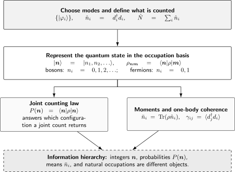
Occupation-number language has an information hierarchy. The chosen mode basis fixes what is counted; $\rho$ fixes both the diagonal counting law $P(\boldsymbol n)$ and possible off-diagonal coherence. Means retain less information than the full joint law.

A Mode Must Be Specified First

Choose an orthonormal basis of the one-particle Hilbert space,

$$\mathcal B = \left\{ \lvert\varphi_i\rangle \right\}.$$

A mode label $i$ may include several quantum numbers:

$$i = (\mathbf k,\sigma,\lambda,\ldots),$$

such as momentum $\mathbf k$, spin projection $\sigma$, band index $\lambda$, lattice site, trap orbital, or polarization. A statement such as “mode $i$ is occupied” is incomplete until this basis and every internal label have been specified.

The corresponding creation and annihilation operators satisfy either bosonic commutators or fermionic anticommutators. To keep formulas common to both cases, this page writes them as $d_i^\dagger$ and $d_i$ whenever the statistics are not being emphasized.

The total number operator is

$$\hat N = \sum_i \hat n_i.$$

If the chosen modes form a complete one-particle basis, this total is independent of an ordinary unitary change of mode basis even though the individual $\hat n_i$ are not.

For distinct orthogonal modes,

$$[\hat n_i,\hat n_j] = 0.$$

The family $\{\hat n_i\}$ can therefore be measured jointly in the idealized projective sense. Its joint eigenvectors are the occupation-number states.

Bosonic and Fermionic Spectra

Bosonic modes

For a bosonic mode,

$$\hat n_i \lvert\ldots,n_i,\ldots\rangle = n_i \lvert\ldots,n_i,\ldots\rangle, \qquad n_i \in \mathbb N_0.$$

Repeated creation in the same mode is allowed. Consequently,

$$\hat n_i^2 \neq \hat n_i$$

as an operator on the full bosonic Fock space. A bosonic mode counter is not a projector.

Fermionic modes

For a fermionic mode, the anticommutation relation gives

$$(c_i^\dagger)^2 = 0,$$

so the only allowed counts are zero and one. The number operator is a projector:

$$\hat n_i^2 = \hat n_i.$$

It follows for every fermionic state that

$$0 \leq \langle\hat n_i\rangle \leq 1.$$

This bound applies to a complete fermionic spin-orbital. An orbital described only by its spatial wavefunction can hold two electrons when its two spin states are treated as distinct modes.

Occupation-Number Configurations

A joint eigenstate is written

$$\lvert\boldsymbol n\rangle = \lvert n_1,n_2,\ldots\rangle.$$

The tuple $\boldsymbol n$ labels a basis vector, not a list of particle identities. For identical particles, the exchange symmetry is already built into the bosonic or fermionic Fock-space construction.

In a fixed-$N$ sector,

$$\sum_i n_i = N.$$

The admissible tuples therefore obey both the statistical restriction on each $n_i$ and the chosen global constraints. A general fixed-number pure state has the expansion

$$\lvert\Psi_N\rangle = \sum_{\boldsymbol n:\,\sum_i n_i=N} C_{\boldsymbol n} \lvert\boldsymbol n\rangle.$$

The coefficients $C_{\boldsymbol n}$ are probability amplitudes. They are not occupations. Their moduli squared become probabilities only for a measurement in this occupation basis.

The canonical pages on Number States and the Occupation-Number Representation give normalization conventions, finite-basis counting, fermionic ordering signs, and matrix construction.

From a Quantum State to a Counting Law

Let $\rho$ be a density operator. The probability of obtaining the complete configuration $\boldsymbol n$ is

$$P(\boldsymbol n) = \langle\boldsymbol n\vert \rho \vert\boldsymbol n\rangle.$$

These probabilities satisfy

$$P(\boldsymbol n) \geq 0, \qquad \sum_{\boldsymbol n} P(\boldsymbol n) = 1.$$

For a pure state,

$$\rho = \lvert\Psi\rangle\langle\Psi\rvert,$$

and therefore

$$P(\boldsymbol n) = \left| \langle\boldsymbol n\vert\Psi\rangle \right|^2.$$

Only the diagonal matrix elements of $\rho$ appear. The full quantum state can also have coherences

$$\rho_{\boldsymbol n\boldsymbol m} = \langle\boldsymbol n\vert \rho \vert\boldsymbol m\rangle, \qquad \boldsymbol n \neq \boldsymbol m.$$

Two states with the same $P(\boldsymbol n)$ can therefore make different predictions for observables that are not diagonal in the chosen occupation basis.

Means, Variances, and Covariances

The mean occupation is

$$\begin{aligned} \overline n_i &= \operatorname{Tr} \left( \rho\hat n_i \right) \\ &= \sum_{\boldsymbol n} n_i P(\boldsymbol n). \end{aligned}$$

The total mean number is

$$\overline N = \langle\hat N\rangle = \sum_i \overline n_i.$$

The variance of one mode is

$$\operatorname{Var}(n_i) = \left\langle \hat n_i^2 \right\rangle - \overline n_i^{\,2},$$

and the covariance of two modes is

$$\operatorname{Cov}(n_i,n_j) = \left\langle \hat n_i\hat n_j \right\rangle - \overline n_i\, \overline n_j.$$

The total-number variance collects both:

$$\operatorname{Var}(N) = \sum_i \operatorname{Var}(n_i) + 2 \sum_{i<j} \operatorname{Cov}(n_i,n_j).$$

Means alone do not determine variances, and one-mode variances do not determine cross-mode correlations. The complete joint distribution $P(\boldsymbol n)$ contains all statistics of observables that are functions of the commuting number operators, but it still does not contain every quantum coherence.

Independent Ideal Modes in Equilibrium

Occupation numbers become especially useful when the Hamiltonian and conserved number are diagonal in the same mode basis:

$$\hat H = \sum_i \epsilon_i \hat n_i, \qquad \hat N = \sum_i \hat n_i.$$

In the grand-canonical ensemble,

$$\rho_{\mathrm{GC}} = \frac{1}{\Xi} e^{-\beta(\hat H-\mu\hat N)}.$$

Because the mode number operators commute,

$$\rho_{\mathrm{GC}} = \bigotimes_i \rho_i.$$

Define the one-mode Boltzmann factor

$$x_i = e^{-\beta(\epsilon_i-\mu)}.$$

The joint counting law factorizes:

$$P(\boldsymbol n) = \prod_i P_i(n_i).$$

Consequently, distinct ideal modes are statistically independent in this ensemble:

$$\operatorname{Cov}(n_i,n_j) = 0, \qquad i\neq j.$$

This factorization depends on both the quadratic diagonal Hamiltonian and the grand-canonical constraint structure. It is not a general property of occupation numbers.

Bosonic Thermal Occupations

For one ideal bosonic mode, $n=0,1,2,\ldots$. Normalizing the geometric series gives

$$P_i^{(B)}(n) = (1-x_i)x_i^n, \qquad 0 \leq x_i < 1.$$

The mean and variance are

$$\overline n_i = \frac{x_i}{1-x_i} = \frac{1}{ e^{\beta(\epsilon_i-\mu)}-1 },$$

and

$$\operatorname{Var}(n_i) = \overline n_i \left( 1+\overline n_i \right).$$

Thus the thermal bosonic mode has fluctuations larger than a Poisson variable with the same mean. The factor $1+\overline n_i$ is often described as Bose enhancement.

Solving for $x_i$ in terms of the mean gives

$$x_i = \frac{\overline n_i}{ 1+\overline n_i },$$

so the entire one-mode geometric distribution is fixed by its mean. This special fact does not imply that an arbitrary many-mode bosonic state is fixed by its list of mean occupations.

The canonical derivation, chemical-potential constraint, and physical limits belong to Bose–Einstein Statistics.

Fermionic Thermal Occupations

For one ideal fermionic mode, only $n=0$ and $n=1$ occur:

$$P_i^{(F)}(0) = \frac{1}{1+x_i}, \qquad P_i^{(F)}(1) = \frac{x_i}{1+x_i}.$$

The mean is

$$\overline n_i = P_i^{(F)}(1) = \frac{x_i}{1+x_i} = \frac{1}{ e^{\beta(\epsilon_i-\mu)}+1 }.$$

Here, and only because a single fermionic mode has binary outcomes, the mean occupation equals the probability that the mode is occupied.

Since $\hat n_i^2=\hat n_i$,

$$\operatorname{Var}(n_i) = \overline n_i \left( 1-\overline n_i \right).$$

The factor $1-\overline n_i$ suppresses fluctuations as the mode approaches unit occupation. This is the local statistical expression of Pauli blocking.

The equilibrium law and its zero-temperature and finite-temperature limits are developed in Fermi–Dirac Statistics.

The Dilute Classical Counting Law

In the Maxwell–Boltzmann regime,

$$\overline n_i \ll 1.$$

For a grand-canonical classical ideal gas, the number assigned to a one-particle state is Poisson distributed:

$$P_i^{(\mathrm{MB})}(n) = e^{-\lambda_i} \frac{\lambda_i^n}{n!}, \qquad \lambda_i = z e^{-\beta\epsilon_i}.$$

Its mean and variance are both $\lambda_i$:

$$\overline n_i = \operatorname{Var}(n_i) = \lambda_i.$$

At low occupation, the bosonic geometric law, the fermionic Bernoulli law, and the classical Poisson law agree at leading order in $\overline n_i$. Their differences first become visible in multiparticle probabilities and fluctuations. The practical classical limit and its domain of validity are developed in the Maxwell–Boltzmann Limit and the Classical Limit of Quantum Statistics.

One-mode law	Allowed values	Mean	Variance
Thermal boson	$0,1,2,\ldots$	$\overline n$	$\overline n(1+\overline n)$
Thermal fermion	$0,1$	$\overline n$	$\overline n(1-\overline n)$
Classical ideal mode	$0,1,2,\ldots$	$\overline n$	$\overline n$

The table compares specific equilibrium probability laws. It must not be read as a classification of every possible bosonic or fermionic state. A bosonic coherent state, for example, has Poisson number statistics even though the quanta are bosons.

Modes Versus Degenerate Energy Levels

A mode is one basis vector. An energy level may contain several orthogonal modes with the same energy. If

$$\epsilon_{r\alpha} = \epsilon_r, \qquad \alpha = 1,\ldots,g_r,$$

then the total population of level $r$ is

$$\hat N_r = \sum_{\alpha=1}^{g_r} \hat n_{r\alpha}.$$

For independent ideal modes,

$$\overline N_r = g_r f(\epsilon_r),$$

where $f$ is the Bose–Einstein or Fermi–Dirac mean occupation of one mode.

Fermionic level statistics

Each of the $g_r$ fermionic modes is Bernoulli distributed with common mean $f_r$. Their sum is binomial:

$$P_F(N_r=m) = \binom{g_r}{m} f_r^m (1-f_r)^{g_r-m},$$

for

$$m = 0,1,\ldots,g_r.$$

The level can therefore contain more than one fermion even though no individual mode can.

Bosonic level statistics

The sum of $g_r$ independent geometric variables has a negative-binomial law:

$$P_B(N_r=m) = \binom{m+g_r-1}{m} (1-x_r)^{g_r} x_r^m.$$

Its mean and variance are

$$\overline N_r = g_r \frac{x_r}{1-x_r},$$

and

$$\operatorname{Var}(N_r) = g_r \frac{x_r}{(1-x_r)^2}.$$

Confusing a mode with a degenerate level is a common source of missing factors of two, especially for electron spin and photon polarization.

Sums and Density-of-States Integrals

Mean thermodynamic quantities are often sums over modes. For example,

$$\overline N = \sum_i f(\epsilon_i),$$

and, for a diagonal ideal Hamiltonian,

$$\overline E = \sum_i \epsilon_i f(\epsilon_i).$$

When the spectrum is sufficiently dense, the mode sum becomes

$$\sum_i F(\epsilon_i) \longrightarrow \int d\epsilon\, g(\epsilon) F(\epsilon),$$

where $g(\epsilon)$ counts one-particle modes per unit energy. Internal degeneracies must be included either in $g(\epsilon)$ or as an explicit sum, but not both.

The function $f(\epsilon)$ is the mean occupation per mode. It is not itself the density of particles in energy space. The latter is

$$\frac{d\overline N}{d\epsilon} = g(\epsilon) f(\epsilon).$$

This distinction is central in the Ideal Bose Gas and Ideal Fermi Gas.

Ensemble Constraints Create Correlations

The grand-canonical ideal-mode law factorizes because $\hat H-\mu\hat N$ is a sum of commuting one-mode terms and particle number may fluctuate. A canonical ensemble instead fixes

$$\sum_i n_i = N.$$

For an ideal gas,

$$P_N(\boldsymbol n) = \frac{1}{Z_N} e^{-\beta\sum_i\epsilon_i n_i} \delta_{\sum_i n_i,N},$$

with the allowed bosonic or fermionic tuples understood. The Kronecker delta couples the modes, so

$$P_N(\boldsymbol n) \neq \prod_i P_i(n_i)$$

in general.

Because $\hat N$ has no fluctuations in a fixed-$N$ ensemble,

$$\operatorname{Var}(N) = 0.$$

Equivalently, for every $i$,

$$\sum_j \operatorname{Cov}(n_i,n_j) = \operatorname{Cov}(n_i,N) = 0.$$

The positive self-variance of a mode must be balanced by cross-mode covariances. Individual cross-covariances are often negative in simple fixed-number problems, but their signs need not be asserted without examining the model and the chosen observables.

A microcanonical energy constraint introduces additional correlations. Ensemble equivalence concerns suitable thermodynamic observables and limits; it does not mean that finite-system joint counting distributions are identical in different ensembles.

Worked Example: One Fermion Shared by Two Modes

Consider a fixed one-particle state

$$\lvert\Psi\rangle = \alpha \lvert1,0\rangle + \beta \lvert0,1\rangle, \qquad |\alpha|^2+|\beta|^2=1.$$

The configuration probabilities are

$$P(1,0) = |\alpha|^2, \qquad P(0,1) = |\beta|^2.$$

The mean occupations are

$$\overline n_1 = |\alpha|^2, \qquad \overline n_2 = |\beta|^2,$$

and

$$\overline n_1+\overline n_2 = 1.$$

Since $n_1n_2=0$ in every allowed configuration,

$$\operatorname{Cov}(n_1,n_2) = - |\alpha|^2|\beta|^2.$$

The negative covariance here comes from the fixed total: if the count is in mode 1, it cannot also be in mode 2.

The relative phase between $\alpha$ and $\beta$ does not appear in $P(n_1,n_2)$ or in the two means. It does appear in off-diagonal one-body coherence, which is why occupation probabilities do not specify the full state.

Basis Dependence

Let a second orthonormal mode basis be related to the first by

$$\lvert\chi_\alpha\rangle = \sum_i U_{i\alpha} \lvert\varphi_i\rangle,$$

where $U$ is unitary. The annihilation operators transform as

$$b_\alpha = \sum_i U_{i\alpha}^* d_i.$$

The new number operator is

$$\begin{aligned} \hat n'_\alpha &= b_\alpha^\dagger b_\alpha \\ &= \sum_{ij} U_{i\alpha} U_{j\alpha}^* d_i^\dagger d_j. \end{aligned}$$

It contains off-diagonal bilinears $d_i^\dagger d_j$ in the old basis. Therefore the new mean occupations cannot generally be reconstructed from the old means $\{\overline n_i\}$ alone.

For example, define

$$b_\pm^\dagger = \frac{ d_1^\dagger \pm d_2^\dagger }{ \sqrt2 }.$$

The one-particle state

$$\lvert\Psi\rangle = \frac{ \lvert1,0\rangle + \lvert0,1\rangle }{ \sqrt2 }$$

has

$$\overline n_1 = \overline n_2 = \frac12$$

in the original basis, but it is exactly

$$\lvert1_+,0_-\rangle$$

in the rotated basis. The same physical state has fractional mean occupations in one basis and definite integer occupation in another.

The Mode Occupations page owns the general basis-change construction. The lesson needed here is that a distribution function such as $f(\epsilon_i)$ presupposes a physically selected mode basis, usually the eigenbasis of an ideal one-body Hamiltonian.

The One-Body Density Matrix

The one-body density matrix in a chosen mode basis is

$$\gamma_{ij} = \left\langle d_j^\dagger d_i \right\rangle.$$

Its diagonal entries are the mean occupations:

$$\gamma_{ii} = \overline n_i.$$

Its off-diagonal entries record one-body coherence between modes. The matrix is Hermitian and positive semidefinite, and

$$\operatorname{Tr}\gamma = \sum_i \overline n_i = \overline N.$$

Under the unitary basis change above,

$$\gamma' = U^\dagger \gamma U.$$

The diagonal of $\gamma$ changes, but its eigenvalues do not.

For the coherent one-particle state in the preceding example,

$$\gamma = \frac12 \begin{pmatrix} 1 & 1\\ 1 & 1 \end{pmatrix}.$$

The corresponding incoherent mixture

$$\rho_{\mathrm{mix}} = \frac12 \lvert1,0\rangle\langle1,0\rvert + \frac12 \lvert0,1\rangle\langle0,1\rvert$$

has the same counting probabilities and the same diagonal means in the original basis, but

$$\gamma_{\mathrm{mix}} = \frac12 \begin{pmatrix} 1 & 0\\ 0 & 1 \end{pmatrix}.$$

A measurement in the rotated basis distinguishes them.

Natural Occupations

Diagonalizing the one-body density matrix gives

$$\gamma \lvert\phi_\alpha^{\mathrm{nat}}\rangle = \nu_\alpha \lvert\phi_\alpha^{\mathrm{nat}}\rangle.$$

The eigenvectors are natural orbitals and the eigenvalues $\nu_\alpha$ are natural occupations. They satisfy

$$\nu_\alpha \geq 0, \qquad \sum_\alpha \nu_\alpha = \overline N.$$

For fermions, the anticommutation relations imply

$$0 \leq \nu_\alpha \leq 1.$$

A pure Slater determinant has natural occupations equal to zero or one. Fractional natural occupations are a common signature that a fermionic state is not a single Slater determinant, although the list of eigenvalues alone does not fully characterize many-body correlations.

Bosonic natural occupations are nonnegative and can exceed one. In the thermodynamic setting, the Penrose–Onsager criterion identifies Bose–Einstein condensation with a largest eigenvalue that scales extensively:

$$\nu_{\max} \sim O(N).$$

That criterion is basis independent because it uses an eigenvalue of $\gamma$, not the diagonal occupation of an arbitrarily chosen orbital. The thermodynamics of the ideal-gas transition belongs to the later Bose–Einstein condensation page.

A natural occupation $\nu_\alpha=0.37$ is not a possible eigenvalue returned by a number measurement. It is a mean occupation of a natural orbital.

One-Body Observables

A one-body operator has the second-quantized form

$$\hat A = \sum_{ij} A_{ij} d_i^\dagger d_j.$$

Its expectation value is

$$\begin{aligned} \langle\hat A\rangle &= \sum_{ij} A_{ij} \gamma_{ji} \\ &= \operatorname{Tr} \left( A\gamma \right). \end{aligned}$$

If $A$ is diagonal in the chosen mode basis,

$$A_{ij} = A_i\delta_{ij},$$

then

$$\langle\hat A\rangle = \sum_i A_i \overline n_i.$$

This is why mean occupations are sufficient for the energy and number of an ideal gas in its energy eigenbasis. If $A$ has off-diagonal matrix elements, the off-diagonal entries of $\gamma$ are also required.

The operator identity and its action on Fock states are developed in One-Body Operators. The many-body application guide treats off-diagonal coherence, transition matrices, dynamics, and active-space truncation.

Higher Moments and Counting Correlations

The one-body density matrix does not determine every number fluctuation. Two-body information enters quantities such as

$$\left\langle \hat n_i\hat n_j \right\rangle$$

and

$$\left\langle \hat n_i (\hat n_i-1) \right\rangle.$$

For a bosonic mode, the normalized equal-mode factorial correlation is

$$g_i^{(2)} = \frac{ \left\langle \hat n_i(\hat n_i-1) \right\rangle }{ \overline n_i^{\,2} },$$

when $\overline n_i\neq0$.

Representative values are:

$$g_i^{(2)} = \begin{cases} 2, & \text{single ideal thermal bosonic mode}, \\ 1, & \text{Poisson number statistics}, \\ 0, & \text{single fermionic mode}. \end{cases}$$

These values describe counting statistics, not particle identity labels. Spatially resolved correlations, field-operator forms, and connected correlators are developed in Correlation Functions Overview.

Generating Functions

For a finite set of commuting mode counters, define the counting characteristic function

$$\chi(\boldsymbol\theta) = \left\langle \exp \left( i \sum_j \theta_j \hat n_j \right) \right\rangle.$$

In terms of the joint probability law,

$$\chi(\boldsymbol\theta) = \sum_{\boldsymbol n} P(\boldsymbol n) e^{i\boldsymbol\theta\cdot\boldsymbol n}.$$

Derivatives at the origin generate moments. For example,

$$\overline n_i = \left. \frac{1}{i} \frac{\partial\chi}{ \partial\theta_i } \right|_{\boldsymbol\theta=0}.$$

Derivatives of

$$K(\boldsymbol\theta) = \ln\chi(\boldsymbol\theta)$$

generate cumulants, including variances and covariances. For independent modes,

$$\chi(\boldsymbol\theta) = \prod_i \chi_i(\theta_i), \qquad K(\boldsymbol\theta) = \sum_i K_i(\theta_i).$$

This is the occupation-number form of full counting statistics. It is useful when a mean and variance are insufficient, as in transport, cold-atom snapshots, and photon counting.

Interacting Systems

Occupation-number basis states remain a valid basis for interacting systems, but they are generally not energy eigenstates. A typical Hamiltonian has

$$\hat H = \sum_{ij} h_{ij} d_i^\dagger d_j + \frac12 \sum_{ijkl} V_{ijkl} d_i^\dagger d_j^\dagger d_l d_k.$$

Off-diagonal one-body terms move particles between modes. Interaction terms can scatter pairs of particles from one configuration to another. A thermal density operator

$$\rho \propto e^{-\beta(\hat H-\mu\hat N)}$$

then need not be diagonal or factorized in the chosen bare-mode occupation basis.

Accordingly, the formulas

$$\overline n_i = \frac{1}{ e^{\beta(\epsilon_i-\mu)} \mp 1 }$$

apply directly only to independent modes of a diagonal quadratic Hamiltonian, or to controlled quasiparticle descriptions with their own assumptions. Interactions may broaden spectral weight, create correlations, and make no single set of bare occupations independently thermal.

There is no contradiction between using an occupation-number basis to diagonalize an interacting Hamiltonian and finding that the eigenvectors are superpositions of many occupation configurations. A basis label need not be a conserved quantum number.

Particle and Quasiparticle Occupations

An ordinary unitary mode change mixes annihilation operators only:

$$b_\alpha = \sum_i U_{i\alpha}^* d_i.$$

A Bogoliubov transformation may mix annihilation and creation operators:

$$\beta_\alpha = \sum_i \left( u_{\alpha i}d_i + v_{\alpha i}d_i^\dagger \right),$$

with signs and conjugations fixed by the bosonic or fermionic convention. The quasiparticle vacuum satisfies

$$\beta_\alpha \lvert\Omega\rangle = 0,$$

but it can have nonzero occupation of the original particles:

$$\langle\Omega| d_i^\dagger d_i |\Omega\rangle \neq 0.$$

This page owns the operator and ensemble bookkeeping of those occupations. Quasiparticles Overview owns the physical criteria that make the $\beta_\alpha$ excitations particle-like and explains why their number need not be an exact conserved charge.

Thus “zero quasiparticles” does not generally mean “zero microscopic particles.” The relevant occupation must always name the operators being counted.

Likewise, a chemical potential couples to a conserved microscopic number or charge. One should not assign an independent chemical potential to a quasiparticle number that is not conserved.

Measurement Interpretation

An ideal joint measurement of the selected mode counters has projectors

$$\Pi_{\boldsymbol n} = \lvert\boldsymbol n\rangle \langle\boldsymbol n\rvert$$

for a nondegenerate occupation basis, and returns $\boldsymbol n$ with probability

$$P(\boldsymbol n) = \operatorname{Tr} \left( \rho\Pi_{\boldsymbol n} \right).$$

Real detectors often measure a coarse-grained count,

$$\hat N_R = \sum_{i\in R} \hat n_i,$$

such as all momenta in a bin, all particles in a spatial region, or both spin states in one site. The probability law of $\hat N_R$ is obtained by summing $P(\boldsymbol n)$ over all configurations with the same coarse-grained total.

Finite efficiency, finite resolution, loss, and interactions during readout can modify the observed counting distribution. Those are properties of the measurement model, not changes to the definition of the occupation-number operator.

Worked Example: A Thermal Bosonic Mode

Suppose

$$x = e^{-\beta(\epsilon-\mu)} = \frac13.$$

Then

$$P(n) = \frac23 \left( \frac13 \right)^n.$$

The first probabilities are

$$P(0) = \frac23, \qquad P(1) = \frac29, \qquad P(2) = \frac{2}{27}.$$

The mean and variance are

$$\overline n = \frac{x}{1-x} = \frac12,$$

and

$$\operatorname{Var}(n) = \overline n(1+\overline n) = \frac34.$$

The mean is one half, even though every outcome is an integer. The probability of two particles is nonzero, so interpreting $\overline n=1/2$ as “a fifty-percent chance of one particle and otherwise zero” would give the wrong distribution.

Worked Example: Same Means, Different States

Consider two bosonic modes and the states

$$\lvert\Psi\rangle = \frac{ \lvert1,0\rangle + \lvert0,1\rangle }{ \sqrt2 },$$

and

$$\rho_{\mathrm{mix}} = \frac12 \lvert1,0\rangle\langle1,0\rvert + \frac12 \lvert0,1\rangle\langle0,1\rvert.$$

Both have

$$\overline n_1 = \overline n_2 = \frac12$$

and the same original-basis counting law:

$$P(1,0) = P(0,1) = \frac12.$$

Yet the coherent state has natural occupations

$$(\nu_1,\nu_2) = (1,0),$$

whereas the mixture has

$$(\nu_1,\nu_2) = \left( \frac12,\frac12 \right).$$

The example separates three levels of information: means, one-basis counting probabilities, and one-body coherence.

Practical Workflow

For an occupation-number calculation:

1. Specify a complete orthonormal set of one-particle modes, including spin or internal labels.
2. State whether the operators are bosonic, fermionic, or quasiparticle operators.
3. Distinguish the operator $\hat n_i$, its integer eigenvalue $n_i$, and its mean $\overline n_i$.
4. State the ensemble and all exact constraints, especially fixed particle number.
5. Check whether the Hamiltonian is diagonal and quadratic in the selected mode operators.
6. Use a product one-mode law only when factorization is justified.
7. Include degeneracy in the mode count exactly once.
8. Use covariances or a generating function when fluctuations matter.
9. Use the one-body density matrix when changing mode basis or evaluating nondiagonal one-body observables.
10. Identify whether a reported occupation is a bare-particle, natural-orbital, or quasiparticle occupation.

Common Mistakes

Treating an occupation number as a probability.
$n_i$ is an integer count. $P(n_i)$ is a probability distribution. $\overline n_i$ is an average of counts.

Interpreting every fractional mean as a fractional particle.
A single ideal number measurement still returns an allowed integer.

Using $\overline n_i$ as the occupancy probability of a bosonic mode.
For bosons, the probability that the mode is nonempty is

$$P(n_i\geq1) = 1-P(0),$$

which need not equal $\overline n_i$.

Forgetting that a mode includes spin.
Pauli exclusion limits each complete fermionic mode to one particle, not each spatial orbital to one particle.

Confusing a mode with a degenerate energy level.
A level occupation is the sum of the occupations of all modes at that energy.

Assuming a list of means determines the state.
It omits mode covariances, higher moments, and coherence.

Assuming ideal grand-canonical modes are always independent.
Fixed-number constraints and interactions correlate occupations.

Applying Bose–Einstein or Fermi–Dirac factors to arbitrary bare modes.
The familiar factors require independent equilibrium modes of a diagonal quadratic Hamiltonian.

Calling natural occupations Fock-state eigenvalues.
Natural occupations are eigenvalues of a one-body density matrix and may be fractional.

Changing mode basis using only old diagonal occupations.
Off-diagonal one-body coherence is generally required.

Confusing zero occupation with zero oscillator energy.
For a harmonic mode, $n=0$ means no quanta, while the Hamiltonian may still include a zero-point term $\hbar\omega/2$.

Assigning a chemical potential to a nonconserved excitation number.
Photons and phonons in ordinary equilibrium have no conserved quasiparticle number and commonly use $\mu=0$.

Exercises

Geometric occupation law

For a bosonic mode with

$$P(n) = (1-x)x^n, \qquad 0\leq x<1,$$

derive $\overline n$ and $\operatorname{Var}(n)$. Express $P(0)$ and $P(n\geq1)$ in terms of $\overline n$.

Solution

The geometric sums give

$$\sum_{n=0}^{\infty} n x^n = \frac{x}{(1-x)^2},$$

and

$$\sum_{n=0}^{\infty} n^2x^n = \frac{x(1+x)}{(1-x)^3}.$$

Therefore

$$\overline n = (1-x) \frac{x}{(1-x)^2} = \frac{x}{1-x},$$

and

$$\begin{aligned} \operatorname{Var}(n) &= \frac{x(1+x)}{(1-x)^2} - \frac{x^2}{(1-x)^2} \\ &= \frac{x}{(1-x)^2} \\ &= \overline n (1+\overline n). \end{aligned}$$

Solving for $x$ gives

$$x = \frac{\overline n}{1+\overline n}.$$

Hence

$$P(0) = 1-x = \frac{1}{1+\overline n},$$

and

$$P(n\geq1) = x = \frac{\overline n}{1+\overline n}.$$

The nonempty probability equals the mean only in the dilute limit.

Fermionic projector identity

Use $\hat n^2=\hat n$ for a single fermionic mode to derive its variance in an arbitrary state. At which mean occupation is the variance largest?

Solution

The projector identity implies

$$\langle\hat n^2\rangle = \langle\hat n\rangle = \overline n.$$

Therefore

$$\operatorname{Var}(n) = \overline n - \overline n^{\,2} = \overline n(1-\overline n).$$

Differentiating with respect to $\overline n$ gives

$$\frac{d}{d\overline n} \operatorname{Var}(n) = 1-2\overline n.$$

The maximum occurs at

$$\overline n = \frac12, \qquad \operatorname{Var}_{\max} = \frac14.$$

This result uses only the binary fermionic spectrum, not thermal equilibrium.

Fixed-number covariance

Two modes contain exactly one particle. Let mode 1 be occupied with probability $p$ and mode 2 with probability $1-p$. Compute all means, variances, and the covariance. Verify $\operatorname{Var}(N)=0$.

Solution

The only configurations are $(1,0)$ and $(0,1)$. Thus

$$\overline n_1 = p, \qquad \overline n_2 = 1-p.$$

Both variables are binary:

$$\operatorname{Var}(n_1) = p(1-p),$$

and

$$\operatorname{Var}(n_2) = p(1-p).$$

Because $n_1n_2=0$ for both configurations,

$$\operatorname{Cov}(n_1,n_2) = - p(1-p).$$

Therefore

$$\begin{aligned} \operatorname{Var}(N) &= \operatorname{Var}(n_1) + \operatorname{Var}(n_2) + 2\operatorname{Cov}(n_1,n_2) \\ &= 0. \end{aligned}$$

Rotate the mode basis

For the one-particle state

$$\lvert\Psi_\phi\rangle = \frac{ \lvert1,0\rangle + e^{i\phi} \lvert0,1\rangle }{ \sqrt2 },$$

define

$$b_\pm^\dagger = \frac{ d_1^\dagger \pm d_2^\dagger }{ \sqrt2 }.$$

Find $\overline n_+$ and $\overline n_-$. Show that the original means do not determine the answer.

Solution

The one-body density matrix in the original basis is

$$\gamma = \frac12 \begin{pmatrix} 1 & e^{-i\phi}\\ e^{i\phi} & 1 \end{pmatrix}.$$

Using the symmetric and antisymmetric mode vectors gives

$$\overline n_+ = \frac{ 1+\cos\phi }{2},$$

and

$$\overline n_- = \frac{ 1-\cos\phi }{2}.$$

For every $\phi$, the original means are

$$\overline n_1 = \overline n_2 = \frac12.$$

The phase appears only in the off-diagonal entries of $\gamma$, so the old diagonal occupations are insufficient for predicting the new ones.

Degenerate fermionic level

A level contains $g=4$ independent fermionic modes, each with mean occupation $f=1/3$ in the grand-canonical ideal gas. Find the mean, variance, and probability of exactly two particles in the level.

Solution

The level population is binomial:

$$N_r \sim \operatorname{Binomial} \left( 4,\frac13 \right).$$

Thus

$$\overline N_r = 4f = \frac43,$$

and

$$\operatorname{Var}(N_r) = 4f(1-f) = \frac89.$$

The probability of exactly two particles is

$$\begin{aligned} P(N_r=2) &= \binom42 \left( \frac13 \right)^2 \left( \frac23 \right)^2 \\ &= \frac{8}{27}. \end{aligned}$$

No mode has more than one fermion, but the fourfold-degenerate level can contain up to four.

One-body observable from the density matrix

In a two-mode basis, let

$$\gamma = \begin{pmatrix} 3/4 & i/4\\ -i/4 & 1/4 \end{pmatrix},$$

and

$$A = \begin{pmatrix} \epsilon & it\\ -it & 2\epsilon \end{pmatrix},$$

where $\epsilon$ and $t$ are real. Compute $\langle\hat A\rangle=\operatorname{Tr}(A\gamma)$. What would be missed by using only the mean occupations?

Solution

Matrix multiplication gives

$$\begin{aligned} \operatorname{Tr}(A\gamma) &= \epsilon \left( \frac34 \right) + 2\epsilon \left( \frac14 \right) + (it) \left( -\frac{i}{4} \right) + (-it) \left( \frac{i}{4} \right) \\ &= \frac{5\epsilon}{4} + \frac{t}{2}. \end{aligned}$$

Using only the diagonal occupations would give $5\epsilon/4$ and miss the coherence contribution $t/2$.

Natural occupations

Find the natural occupations of

$$\gamma = \begin{pmatrix} 1/2 & q\\ q^* & 1/2 \end{pmatrix}.$$

What conditions on $q$ follow for a one-particle fermionic density matrix?

Solution

The characteristic polynomial gives eigenvalues

$$\nu_\pm = \frac12 \pm |q|.$$

Positivity requires

$$|q| \leq \frac12.$$

The trace is one, as required for one particle. The fermionic upper bound $\nu_\pm\leq1$ gives the same restriction.

At $|q|=1/2$, the eigenvalues are $(1,0)$ and the one-body state is pure. At $q=0$, they are $(1/2,1/2)$ and there is no one-body coherence in this basis.

Bare particles in a bosonic quasiparticle vacuum

For one bosonic mode, consider

$$\beta = u a + v a^\dagger,$$

with

$$|u|^2-|v|^2=1.$$

If $\beta\lvert\Omega\rangle=0$, show that the bare-particle mean is

$$\langle\Omega| a^\dagger a |\Omega\rangle = |v|^2.$$

Solution

The inverse transformation can be written

$$a = u^*\beta - v\beta^\dagger.$$

Therefore

$$a^\dagger = u\beta^\dagger - v^*\beta.$$

Multiplying and taking the quasiparticle-vacuum expectation value leaves only the term containing $\beta\beta^\dagger$:

$$\begin{aligned} \langle a^\dagger a\rangle &= |v|^2 \langle\Omega| \beta\beta^\dagger |\Omega\rangle \\ &= |v|^2. \end{aligned}$$

The quasiparticle vacuum contains no $\beta$ quanta but has a nonzero mean occupation of the original $a$ particles.

Cross-Links

• Occupation-Number Basis — canonical construction of bosonic and fermionic Fock basis states.
• Mode Occupations — what a mode is and how occupations change under basis rotations.
• Number Operators — spectra, commutators, and number conservation.
• One-Body Operators — why one-body expectations require the one-body density matrix.
• One-Body Operators in Many-Body Models — practical matrix construction, transition densities, dynamics, and effective-operator cautions.
• Occupation-Number Representation — finite basis construction, counting, matrix elements, and computation.
• Grand-Canonical Ensemble — the ensemble in which independent ideal modes factorize.
• Fluctuations and Susceptibilities — thermodynamic meaning of number fluctuations and response.
• Bose–Einstein Statistics and Fermi–Dirac Statistics — canonical equilibrium occupation laws.
• Correlation Functions Overview — one-body density matrices, density correlations, and connected correlators.

References

• R. K. Pathria and P. D. Beale, Statistical Mechanics, 4th ed., Academic Press (2021) — quantum ideal gases, ensembles, and occupation-number distributions.
• K. Huang, Statistical Mechanics, 2nd ed., Wiley (1987) — standard treatment of Bose, Fermi, and classical occupation laws.
• A. L. Fetter and J. D. Walecka, Quantum Theory of Many-Particle Systems, Dover (2003) — second-quantized many-body formalism and one-body density matrices.
• J. W. Negele and H. Orland, Quantum Many-Particle Systems, CRC Press (1998) — occupation-number methods, ensembles, and correlation functions.
• P. Coleman, Introduction to Many-Body Physics, Cambridge University Press (2015) — modern many-body notation and quasiparticle reasoning.
• A. J. Coleman, “Structure of Fermion Density Matrices”, Reviews of Modern Physics 35, 668–686 (1963) — foundational analysis of fermionic reduced density matrices and occupation constraints.
• O. Penrose and L. Onsager, “Bose–Einstein Condensation and Liquid Helium”, Physical Review 104, 576–584 (1956) — basis-independent condensation criterion from the one-body density matrix.