Sommerfeld Expansion

The Sommerfeld expansion is the low-temperature asymptotic expansion of an energy integral weighted by the Fermi–Dirac occupation. Its standard form turns

$$I(T,\mu) = \int_{\epsilon_0}^{\infty} d\epsilon\, \varphi(\epsilon) f(\epsilon;\mu,T)$$

into a zero-temperature integral plus derivatives of the smooth factor $\varphi$ evaluated at the chemical potential.

Here

$$f(\epsilon;\mu,T) = \frac{1}{ e^{(\epsilon-\mu)/(k_{\mathrm B}T)}+1 }$$

is the Fermi–Dirac distribution, and $\epsilon_0$ is the lower edge of the one-particle spectrum or band under consideration.

The method works because a low-temperature Fermi function differs from the step function $\Theta(\mu-\epsilon)$ only in a narrow energy window of width $O(k_{\mathrm B}T)$. If $\varphi$ varies smoothly across that window, only its local derivatives near $\epsilon=\mu$ matter.

The Sommerfeld expansion is local in energy but global in bookkeeping. The coefficients come from the thermal window near $\mu$, while a fixed-particle-number calculation must also determine how $\mu$ shifts with temperature.

This page is the canonical home for the mathematical expansion, its assumptions, the fixed-$N$ correction, and its application to low-temperature energy and heat capacity. Degenerate Fermi Gas owns the physical regime, Fermi Surface owns the momentum-space geometry, and Ideal Fermi Gas owns the complete three-dimensional model.

Notation and Scope

It is useful to abbreviate the thermal energy by

$$\tau \equiv k_{\mathrm B}T.$$

The expansion parameter is not temperature by itself. It is a dimensionless ratio such as

$$\frac{\tau}{E_{\mathrm{var}}} \ll 1,$$

where $E_{\mathrm{var}}$ is the smallest energy scale over which $\varphi$ changes appreciably near $\mu$. The distance to a band edge or singularity can be an equally important scale.

Unless stated otherwise, assume:

• $T>0$ and $\mu$ lies inside a continuum of states;
• $\mu-\epsilon_0\gg\tau$;
• $\varphi$ is sufficiently differentiable near $\mu$;
• $\varphi$ and its derivatives grow slowly enough for the integrals to exist;
• no discontinuity, gap edge, or van Hove singularity lies within the thermal window;
• the continuum integral is appropriate, so the relevant level spacing is much smaller than $\tau$.

The Asymptotic Analysis page explains why an asymptotic series need not converge to be useful.

Statement of the Expansion

Under the stated assumptions,

$$\begin{aligned} I(T,\mu) ={}& \int_{\epsilon_0}^{\mu} d\epsilon\, \varphi(\epsilon) \\ &+ \frac{\pi^2}{6} \tau^2 \varphi'(\mu) \\ &+ \frac{7\pi^4}{360} \tau^4 \varphi'''(\mu) \\ &+ O(\tau^6). \end{aligned}$$

Only odd derivatives of $\varphi$ appear, and only even powers of $T$ occur. The reason is a particle–hole symmetry of the thermal broadening kernel about $\epsilon=\mu$.

The general formal series is

$$\begin{aligned} I(T,\mu) \sim{}& \int_{\epsilon_0}^{\mu} d\epsilon\, \varphi(\epsilon) \\ &+ \sum_{n=1}^{\infty} c_{2n} \tau^{2n} \varphi^{(2n-1)}(\mu), \end{aligned}$$

with

$$c_{2n} = 2 \left( 1-2^{1-2n} \right) \zeta(2n).$$

The first coefficients are

$$\begin{array}{c|c} n & c_{2n} \\ \hline 1 & \pi^2/6 \\ 2 & 7\pi^4/360 \\ 3 & 31\pi^6/15120 \end{array}$$

The symbol $\sim$ emphasizes asymptotic equality as $\tau$ tends to zero under fixed smoothness and scale assumptions.

The Thermal Window

Two related functions encode the low-temperature localization. The occupation $f$ smooths the zero-temperature step, while

$$\begin{aligned} w_T(\epsilon) &\equiv -\frac{\partial f}{\partial\epsilon} \\ &= \frac{1}{4\tau} \operatorname{sech}^2 \left( \frac{\epsilon-\mu}{2\tau} \right) \end{aligned}$$

is a positive, normalized kernel concentrated near $\mu$.

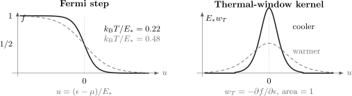
On a fixed energy scale $E_*$, cooling sharpens the Fermi step and narrows $w_T=-\partial f/\partial\epsilon$. The kernel keeps unit area, so its height grows as its width shrinks.

On the full energy line,

$$\int_{-\infty}^{\infty} d\epsilon\, w_T(\epsilon) = 1.$$

Its odd central moments vanish. The first nonzero even moments are

$$\int_{-\infty}^{\infty} d\epsilon\, (\epsilon-\mu)^2 w_T(\epsilon) = \frac{\pi^2}{3} \tau^2$$

and

$$\int_{-\infty}^{\infty} d\epsilon\, (\epsilon-\mu)^4 w_T(\epsilon) = \frac{7\pi^4}{15} \tau^4.$$

Thus $w_T$ approaches the Dirac delta distribution as $T\to0$:

$$w_T(\epsilon) \longrightarrow \delta(\epsilon-\mu).$$

The Sommerfeld expansion refines this delta-kernel limit by retaining its even moments.

Derivation from the Smeared Step

Define the zero-temperature contribution at the same value of $\mu$:

$$I_0(\mu) = \int_{\epsilon_0}^{\mu} d\epsilon\, \varphi(\epsilon).$$

The thermal correction is

$$\begin{aligned} \Delta I ={}& I(T,\mu)-I_0(\mu) \\ ={}& \int_{\mu}^{\infty} d\epsilon\, \varphi(\epsilon)f(\epsilon) \\ &- \int_{\epsilon_0}^{\mu} d\epsilon\, \varphi(\epsilon) \left[1-f(\epsilon)\right]. \end{aligned}$$

The first term counts thermally occupied states above $\mu$; the second subtracts holes created below $\mu$.

Set

$$x = \frac{|\epsilon-\mu|}{\tau}.$$

Using

$$f(\mu+\tau x) = 1-f(\mu-\tau x) = \frac{1}{e^x+1},$$

and extending the lower-side $x$ integral to infinity gives

$$\Delta I = \tau \int_0^{\infty} dx\, \frac{ \varphi(\mu+\tau x) - \varphi(\mu-\tau x) }{e^x+1}$$

up to an endpoint correction exponentially small in $(\mu-\epsilon_0)/\tau$ under the usual regularity assumptions.

Taylor expansion about $\mu$ yields

$$\begin{aligned} &\varphi(\mu+\tau x) - \varphi(\mu-\tau x) \\ &\qquad= 2 \sum_{n=1}^{\infty} \frac{ \varphi^{(2n-1)}(\mu) }{(2n-1)!} (\tau x)^{2n-1}. \end{aligned}$$

Even derivatives cancel because the expression is antisymmetric under $x\mapsto-x$.

The required Fermi moments are

$$\int_0^{\infty} dx\, \frac{x^{s-1}}{e^x+1} = \left(1-2^{1-s}\right) \Gamma(s) \zeta(s),$$

for the values $s=2,4,6,\ldots$ used here. Substituting $s=2n$ cancels $\Gamma(2n)=(2n-1)!$ and gives

$$c_{2n} = 2 \left(1-2^{1-2n}\right) \zeta(2n).$$

This completes the formal derivation.

Derivation with the Kernel

The derivative-kernel form is often more efficient. Introduce an antiderivative

$$\Phi(\epsilon) = \int_{\epsilon_0}^{\epsilon} d\epsilon'\, \varphi(\epsilon').$$

Integration by parts gives

$$I(T,\mu) = \int_{\epsilon_0}^{\infty} d\epsilon\, \Phi(\epsilon) w_T(\epsilon),$$

provided the boundary terms vanish. Expand $\Phi$ about $\mu$:

$$\Phi(\epsilon) = \sum_{r=0}^{\infty} \frac{ \Phi^{(r)}(\mu) }{r!} (\epsilon-\mu)^r.$$

Only even moments of $w_T$ survive. Since

$$\Phi(\mu) = \int_{\epsilon_0}^{\mu} d\epsilon\, \varphi(\epsilon)$$

and

$$\Phi^{(2n)}(\mu) = \varphi^{(2n-1)}(\mu),$$

the same series follows immediately.

This form also gives the useful companion rule

$$\begin{aligned} &\int_{-\infty}^{\infty} d\epsilon\, \Psi(\epsilon) w_T(\epsilon) \\ &\qquad= \Psi(\mu) + \frac{\pi^2}{6} \tau^2 \Psi''(\mu) \\ &\qquad\quad+ \frac{7\pi^4}{360} \tau^4 \Psi^{(4)}(\mu) + O(\tau^6). \end{aligned}$$

Transport and response calculations often begin in this $-\partial f/\partial\epsilon$ form.

What Controls the Approximation

The mnemonic $T\ll T_{\mathrm F}$ is sufficient for a smooth free-particle density of states, but it is not the general criterion. Several independent checks are needed.

Smoothness near the chemical potential

For a truncation through $\tau^{2M}$, the derivatives of $\varphi$ needed through order $2M-1$ must exist and remain controlled in an energy neighborhood of width several $\tau$ around $\mu$.

A practical variation scale is

$$E_r \sim \left| \frac{ \varphi^{(r)}(\mu) }{ \varphi^{(r+1)}(\mu) } \right|,$$

when the ratio is meaningful. One needs $\tau$ small compared with the relevant $E_r$.

Distance from spectral edges

For a lower edge $\epsilon_0$, require

$$\mu-\epsilon_0 \gg \tau.$$

For a finite band with upper edge $\epsilon_1$, also require

$$\epsilon_1-\mu \gg \tau.$$

Otherwise the thermal kernel samples an edge and the extension to an infinite $x$ range is not legitimate.

Absence of nearby singularities

The ordinary series can fail when the density of states has a cusp, jump, logarithmic divergence, or power-law singularity at $\mu$. Nonanalytic corrections such as $T^2\ln T$, fractional powers, or edge-controlled exponentials may replace the regular even-power series.

Continuum resolution

The expansion acts on an integral. In a finite system with mean one-particle level spacing $\Delta$, the smooth continuum approximation additionally needs

$$\Delta \ll \tau.$$

If $\tau\lesssim\Delta$, individual levels, shell effects, parity effects, or Schottky-like crossovers can dominate.

Temperature-independent smooth factor

If $\varphi(\epsilon,T)$ depends explicitly on temperature, the Sommerfeld series expands only the Fermi weighting. The explicit $T$ dependence must be retained and differentiated separately.

Algebraic and Exponential Corrections

The Sommerfeld series captures corrections in powers of $\tau$. It generally omits terms exponentially small in the distance from $\mu$ to a spectral edge.

For example,

$$\int_0^{\infty} d\epsilon\, f(\epsilon;\mu,T) = \tau \ln \left(1+e^{\mu/\tau}\right).$$

When $\mu/\tau\gg1$,

$$\begin{aligned} \tau \ln \left(1+e^{\mu/\tau}\right) &= \mu + \tau \ln \left(1+e^{-\mu/\tau}\right) \\ &= \mu + O \left( \tau e^{-\mu/\tau} \right). \end{aligned}$$

Because $\varphi(\epsilon)=1$ has vanishing odd derivatives, the algebraic Sommerfeld series stops at $\mu$. The remaining correction is not zero; it is beyond all orders in $\tau$.

Fixed Chemical Potential and Fixed Particle Number

The distinction between fixed $\mu$ and fixed $N$ is the most important bookkeeping issue in applications.

For a density of states $D(\epsilon)$ that counts all included internal components, the mean particle number is

$$N(T,\mu) = \int_{\epsilon_0}^{\infty} d\epsilon\, D(\epsilon) f(\epsilon;\mu,T).$$

At fixed $\mu$,

$$\begin{aligned} N(T,\mu) ={}& \int_{\epsilon_0}^{\mu} d\epsilon\, D(\epsilon) \\ &+ \frac{\pi^2}{6} \tau^2 D'(\mu) + O(\tau^4). \end{aligned}$$

Thus the particle number generally changes with temperature in the grand canonical ensemble.

At fixed $N$, define the Fermi energy $\epsilon_{\mathrm F}$ by

$$N = \int_{\epsilon_0}^{\epsilon_{\mathrm F}} d\epsilon\, D(\epsilon).$$

Write

$$\mu(T) = \epsilon_{\mathrm F} + \delta\mu(T).$$

Expanding the number constraint to order $\tau^2$ gives

$$0 = D_{\mathrm F}\,\delta\mu + \frac{\pi^2}{6} \tau^2 D'_{\mathrm F} + O(\tau^4),$$

where

$$D_{\mathrm F} \equiv D(\epsilon_{\mathrm F}), \qquad D'_{\mathrm F} \equiv D'(\epsilon_{\mathrm F}).$$

Therefore

$$\delta\mu(T) = -\frac{\pi^2}{6} \tau^2 \frac{D'_{\mathrm F}}{D_{\mathrm F}} + O(\tau^4).$$

The sign is controlled by the local slope of the density of states:

• if $D'_{\mathrm F}>0$, then $\mu$ decreases;
• if $D'_{\mathrm F}<0$, then $\mu$ increases;
• if $D'_{\mathrm F}=0$, the $T^2$ shift vanishes.

The Chemical Potential page gives the broader thermodynamic meaning of this adjustment.

Energy at Fixed Particle Number

For noninteracting particles with one-particle energy $\epsilon$,

$$U(T,\mu) = \int_{\epsilon_0}^{\infty} d\epsilon\, \epsilon D(\epsilon) f(\epsilon;\mu,T).$$

At fixed $\mu$, apply the expansion with

$$\varphi_U(\epsilon) = \epsilon D(\epsilon).$$

At fixed $N$, however, $\mu$ also shifts. Expanding around $\epsilon_{\mathrm F}$ gives

$$\begin{aligned} U(T,N)-U_0 ={}& \epsilon_{\mathrm F}D_{\mathrm F} \delta\mu \\ &+ \frac{\pi^2}{6} \tau^2 \left[ D_{\mathrm F} + \epsilon_{\mathrm F}D'_{\mathrm F} \right] \\ &+ O(\tau^4). \end{aligned}$$

Substituting the fixed-number shift cancels the terms proportional to $D'_{\mathrm F}$:

$$U(T,N)-U_0 = \frac{\pi^2}{6} D_{\mathrm F} \tau^2 + O(\tau^4).$$

The constant-volume heat capacity at fixed particle number is therefore

$$\begin{aligned} C_{V,N} &= \left( \frac{\partial U}{\partial T} \right)_{V,N} \\ &= \frac{\pi^2}{3} D_{\mathrm F} k_{\mathrm B}^2T + O(T^3). \end{aligned}$$

This result is universal within the smooth noninteracting setting: the leading coefficient depends on the density of one-particle states at the Fermi energy, not on its slope.

Entropy and Free Energy

Define the Sommerfeld coefficient

$$\gamma \equiv \frac{\pi^2}{3} k_{\mathrm B}^2 D_{\mathrm F}.$$

Then, at fixed $N$ and $V$,

$$C_{V,N} = \gamma T + O(T^3).$$

Because $S(0)=0$ for a nondegenerate many-body ground state and

$$C_{V,N} = T \left( \frac{\partial S}{\partial T} \right)_{V,N},$$

the entropy is

$$S(T,N) = \gamma T + O(T^3).$$

The Helmholtz free energy follows from $F=U-TS$:

$$F(T,N) = U_0 - \frac{\gamma}{2} T^2 + O(T^4).$$

Equivalently,

$$F(T,N) = U_0 - \frac{\pi^2}{6} D_{\mathrm F} \tau^2 + O(\tau^4).$$

These relations connect the expansion to the Thermodynamic Potentials page.

Grand Potential Form

For fixed $\mu$, the grand potential is

$$\Omega(T,\mu) = -\tau \int_{\epsilon_0}^{\infty} d\epsilon\, D(\epsilon) \ln \left[ 1+e^{-(\epsilon-\mu)/\tau} \right].$$

Since

$$N = - \left( \frac{\partial\Omega}{\partial\mu} \right)_{T,V},$$

integrating the Sommerfeld expansion for $N$ with respect to $\mu$ gives

$$\begin{aligned} \Omega(T,\mu) ={}& \Omega_0(\mu) - \frac{\pi^2}{6} \tau^2 D(\mu) \\ &- \frac{7\pi^4}{360} \tau^4 D''(\mu) + O(\tau^6), \end{aligned}$$

up to a $\mu$-independent integration constant fixed by the empty-band limit. This form is convenient when pressure, entropy, and number are generated from $\Omega$.

Worked Example: Three-Dimensional Free Gas

For a uniform nonrelativistic gas in three dimensions,

$$D(\epsilon) = A\epsilon^{1/2},$$

where $A$ includes volume and internal degeneracy. Hence

$$\frac{D'_{\mathrm F}}{D_{\mathrm F}} = \frac{1}{2\epsilon_{\mathrm F}}.$$

The fixed-number chemical potential is

$$\begin{aligned} \mu(T) &= \epsilon_{\mathrm F} - \frac{\pi^2}{12} \frac{\tau^2}{\epsilon_{\mathrm F}} + O \left( \frac{\tau^4}{\epsilon_{\mathrm F}^3} \right) \\ &= \epsilon_{\mathrm F} \left[ 1- \frac{\pi^2}{12} \left( \frac{T}{T_{\mathrm F}} \right)^2 + O \left( \frac{T^4}{T_{\mathrm F}^4} \right) \right], \end{aligned}$$

where $k_{\mathrm B}T_{\mathrm F}=\epsilon_{\mathrm F}$.

The zero-temperature state count gives

$$D_{\mathrm F} = \frac{3N}{2\epsilon_{\mathrm F}}.$$

Therefore

$$U(T)-U_0 = \frac{\pi^2}{4} N \frac{\tau^2}{\epsilon_{\mathrm F}} + O \left( N\frac{\tau^4}{\epsilon_{\mathrm F}^3} \right)$$

and

$$\frac{C_{V,N}}{Nk_{\mathrm B}} = \frac{\pi^2}{2} \frac{T}{T_{\mathrm F}} + O \left( \frac{T^3}{T_{\mathrm F}^3} \right).$$

The Fermi Momentum and Fermi Energy page derives the state-counting formulas behind $D_{\mathrm F}$.

Worked Example: Constant Density of States

In an ideal two-dimensional quadratic band,

$$D(\epsilon) = D_0$$

above the band bottom. The algebraic fixed-number shift vanishes because $D'(\epsilon)=0$.

The number equation can be integrated exactly:

$$N = D_0\tau \ln \left( 1+e^{\mu/\tau} \right).$$

Defining $\epsilon_{\mathrm F}=N/D_0$ gives

$$\mu(T) = \tau \ln \left( e^{\epsilon_{\mathrm F}/\tau}-1 \right).$$

Equivalently,

$$\mu(T) = \epsilon_{\mathrm F} + \tau \ln \left( 1-e^{-\epsilon_{\mathrm F}/\tau} \right).$$

Thus

$$\mu(T)-\epsilon_{\mathrm F} \sim -\tau e^{-\epsilon_{\mathrm F}/\tau}.$$

The absence of a $T^2$ term does not make $\mu$ exactly temperature independent. The leading shift is exponentially small and therefore invisible to every algebraic order of the Sommerfeld series.

Power-Law Density of States

Suppose near the Fermi energy

$$D(\epsilon) = A\epsilon^{\alpha},$$

with $\epsilon_{\mathrm F}$ well above the lower edge. Then

$$\frac{D'_{\mathrm F}}{D_{\mathrm F}} = \frac{\alpha}{\epsilon_{\mathrm F}},$$

so

$$\frac{ \mu(T)-\epsilon_{\mathrm F} }{\epsilon_{\mathrm F}} = -\frac{\pi^2}{6} \alpha \left( \frac{T}{T_{\mathrm F}} \right)^2 + O \left( \frac{T^4}{T_{\mathrm F}^4} \right).$$

For a quadratic dispersion in $d$ dimensions,

$$\alpha = \frac{d}{2}-1.$$

The leading shift is therefore positive in one dimension, exponentially small rather than algebraic in the ideal two-dimensional continuum, and negative in three dimensions. The one-dimensional formula still requires $\tau\ll\epsilon_{\mathrm F}$ because the density of states diverges at the band edge. Low-Dimensional Quantum Gases owns the corresponding state counting and physical dimensionality analysis.

Why the Heat Capacity Is Linear

The expansion supplies a quantitative form of the thermally active-shell picture. The number of states whose occupations change appreciably is of order

$$N_{\mathrm{active}} \sim D_{\mathrm F}\tau.$$

Each particle–hole excitation carries an energy of order $\tau$, so

$$U(T)-U_0 \sim D_{\mathrm F}\tau^2.$$

Differentiation then gives

$$C_V \sim D_{\mathrm F}k_{\mathrm B}^2T.$$

The Sommerfeld calculation fixes the numerical coefficient $\pi^2/3$ and shows why the slope of the density of states cancels at fixed particle number.

In a conventional Fermi liquid, the same structure survives with a quasiparticle density of states and interaction-renormalized parameters. The bare ideal-gas formula should not be assigned unchanged to a strongly correlated or non-Fermi-liquid state.

When the Ordinary Expansion Fails

Chemical potential near a band edge

If $\mu-\epsilon_0=O(\tau)$, the lower endpoint lies inside the thermal window. The result depends on the full edge shape, and the replacement of the finite lower limit by $-\infty$ is invalid.

This is common near dilute-band thresholds and during dimensional crossover.

Singular density of states

At a van Hove singularity, $D(\epsilon)$ is not smooth on the required scale. Derivatives such as $D'(\mu)$ may diverge, and the displayed coefficients cease to organize the answer. One must integrate the singular local form directly or use a uniform asymptotic treatment.

Gapped systems

When $\mu$ lies in a true gap, there is no Fermi surface and no smooth nonzero $D_{\mathrm F}$. Low-temperature excitations are commonly activated:

$$C_V \propto e^{-\Delta/\tau}$$

up to prefactors. A power-series Sommerfeld expansion about $\mu$ does not describe that physics.

Discrete spectra

For $\tau$ below the level spacing, a sum over exact levels must replace the continuum density-of-states integral. Oscillatory or shell corrections need not be small even when $T$ is small compared with a bulk Fermi temperature.

Temperature-dependent quasiparticles

If the spectral density, self-energy, effective mass, or band energies vary appreciably with temperature, expanding only the occupation misses additional terms. Their origin should be separated from ordinary Fermi smearing.

A Reliable Calculation Workflow

1. Write the observable as a Fermi-weighted energy integral or a $w_T$-weighted integral.
2. Identify the smooth factor $\varphi$ or $\Psi$, including all density-of-states and degeneracy factors.
3. State whether $\mu$ or $N$ is held fixed.
4. Locate the nearest band edge, singularity, gap, and discrete-level scale.
5. Compare those scales with $\tau=k_{\mathrm B}T$.
6. Expand only to the order supported by the available derivatives and desired accuracy.
7. If $N$ is fixed, solve the number constraint before substituting into other observables.
8. Check units, limiting behavior, and the sign of the correction.

For numerical work, compare the truncated series against direct quadrature at representative temperatures. The optimal number of terms can decrease once higher derivatives grow rapidly.

Common Mistakes

Replacing $\mu(T)$ by $\epsilon_{\mathrm F}$ too early.
This loses the fixed-number correction and generally gives a wrong energy coefficient, even though the final leading heat capacity has a simple form.

Using fixed-$\mu$ and fixed-$N$ derivatives interchangeably.
The ensembles impose different constraints. State the variables held fixed whenever differentiating.

Applying the expansion at a singularity.
A large or divergent derivative is a warning that the smoothness assumption has failed, not evidence for an enormous regular coefficient.

Forgetting an endpoint.
The condition $\mu-\epsilon_0\gg\tau$ is part of the method. It is not optional notation.

Calling omitted exponential terms zero.
A result can vanish to every algebraic order while remaining nonzero as $e^{-E/\tau}$.

Expanding the Fermi function as an ordinary Taylor series in $T$.
The limit is singular at $\epsilon=\mu$. The controlled procedure expands the smooth factor across the localized thermal kernel.

Dropping degeneracy conventions.
$D_{\mathrm F}$ may be per spin, per internal component, per volume, or total. The same convention must be used in $N$, $U$, and $C_V$.

Assuming the series converges.
It is normally used as a low-temperature asymptotic expansion. More terms are not automatically better.

Ignoring explicit temperature dependence in $\varphi$.
Band shifts, interactions, and scattering rates can contribute additional powers of $T$.

Using the ideal-gas coefficient for every metal.
Measured linear heat capacity can include quasiparticle mass renormalization and other interaction effects. The relation to the bare band density of states is model dependent.

Canonical Boundaries and Connections

• Fermi–Dirac Statistics owns the occupation law and its limits.
• Degenerate Fermi Gas owns the physical interpretation of the low-temperature regime and Pauli blocking.
• Fermi Surface owns the geometry and local kinematics of gapless fermionic excitations.
• Ideal Fermi Gas owns the full three-dimensional equation of state and model-specific thermodynamics.
• Fermi Momentum and Fermi Energy owns dimension-dependent state counting and Fermi scales.
• Density of States: First Encounter introduces continuum state counting.
• Asymptotic Analysis owns general asymptotic-series concepts and remainder logic.
• Thermodynamic Potentials owns ensemble-dependent derivatives and Legendre transforms.
• Heat Capacity and Thermodynamics owns experimental calorimetry, component separation, entropy integration, and material inference from a measured linear term.

Summary

For a smooth $\varphi$ and a chemical potential far from spectral edges,

$$\begin{aligned} \int_{\epsilon_0}^{\infty} d\epsilon\, \varphi(\epsilon)f(\epsilon) ={}& \int_{\epsilon_0}^{\mu} d\epsilon\, \varphi(\epsilon) \\ &+ \frac{\pi^2}{6} \tau^2\varphi'(\mu) \\ &+ \frac{7\pi^4}{360} \tau^4\varphi'''(\mu) + O(\tau^6). \end{aligned}$$

At fixed particle number,

$$\mu(T)-\epsilon_{\mathrm F} = -\frac{\pi^2}{6} \tau^2 \frac{D'_{\mathrm F}}{D_{\mathrm F}} + O(\tau^4),$$

and the leading heat capacity is

$$C_{V,N} = \frac{\pi^2}{3} D_{\mathrm F} k_{\mathrm B}^2T + O(T^3).$$

These formulas are powerful because they reduce a thermal integral to local information at the Fermi energy. Their reliability depends on checking smoothness, endpoints, ensemble constraints, and continuum resolution before using the coefficients.

References

• A. Sommerfeld, “Zur Elektronentheorie der Metalle auf Grund der Fermischen Statistik. I. Teil”, Zeitschrift für Physik 47, 1–32 (1928) — original application of Fermi statistics to electrons in metals.
• A. Sommerfeld, “Zur Elektronentheorie der Metalle auf Grund der Fermischen Statistik. II. Teil”, Zeitschrift für Physik 47, 43–60 (1928) — continuation covering thermoelectric and magnetic transport effects.
• NIST Digital Library of Mathematical Functions, §25.12(iii), Fermi–Dirac and Bose–Einstein Integrals — definitions, normalization conventions, and relations to polylogarithms.
• N. W. Ashcroft and N. D. Mermin, Solid State Physics, Holt, Rinehart and Winston (1976), Chapters 2 and 3 — free-electron thermodynamics and low-temperature expansion.
• R. K. Pathria and P. D. Beale, Statistical Mechanics, 3rd ed., Elsevier (2011), Chapter 8 — systematic treatment of ideal Fermi gases and the Sommerfeld lemma.
• L. D. Landau and E. M. Lifshitz, Statistical Physics, Part 1, 3rd ed., Butterworth-Heinemann (1980), §§57–58 — degenerate ideal Fermi gases and low-temperature thermodynamics.
• K. Huang, Statistical Mechanics, 2nd ed., Wiley (1987), Chapter 12 — Fermi gas, density of states, and degenerate limit.
• G. D. Mahan, Many-Particle Physics, 3rd ed., Kluwer Academic/Plenum (2000) — low-energy Fermi systems and response integrals weighted by the Fermi window.

Exercises

Derive the first two coefficients

Starting from

$$\Delta I = \tau \int_0^{\infty} dx\, \frac{ \varphi(\mu+\tau x) - \varphi(\mu-\tau x) }{e^x+1},$$

derive the coefficients of $\tau^2\varphi'(\mu)$ and $\tau^4\varphi'''(\mu)$.

Solution

Expand the numerator:

$$\begin{aligned} &\varphi(\mu+\tau x) - \varphi(\mu-\tau x) \\ &\qquad= 2\tau x\varphi'(\mu) + \frac{2\tau^3x^3}{3!} \varphi'''(\mu) + O(\tau^5). \end{aligned}$$

The needed moments are

$$\int_0^{\infty} dx\, \frac{x}{e^x+1} = \frac{\pi^2}{12}$$

and

$$\int_0^{\infty} dx\, \frac{x^3}{e^x+1} = \frac{7\pi^4}{120}.$$

Therefore

$$2 \left( \frac{\pi^2}{12} \right) = \frac{\pi^2}{6}$$

and

$$\frac{2}{3!} \left( \frac{7\pi^4}{120} \right) = \frac{7\pi^4}{360}.$$

Identify a beyond-all-orders correction

Evaluate

$$I_0(T,\mu) = \int_0^{\infty} d\epsilon\, f(\epsilon;\mu,T)$$

exactly. Show that the Sommerfeld series has no algebraic correction to $\mu$, and find the leading omitted term for $\mu/\tau\gg1$.

Solution

An antiderivative gives

$$I_0(T,\mu) = \tau \ln \left( 1+e^{\mu/\tau} \right).$$

Rewrite this as

$$I_0(T,\mu) = \mu + \tau \ln \left( 1+e^{-\mu/\tau} \right).$$

For $\mu/\tau\gg1$,

$$I_0(T,\mu) = \mu + \tau e^{-\mu/\tau} + O \left( \tau e^{-2\mu/\tau} \right).$$

The smooth factor is $\varphi=1$, whose odd derivatives vanish. Hence every algebraic Sommerfeld correction is zero, while the endpoint leaves an exponentially small term.

Derive the fixed-number chemical-potential shift

Let $D(\epsilon)$ be smooth and nonzero at $\epsilon_{\mathrm F}$. Starting from the number constraint, derive the leading shift of $\mu(T)$ at fixed $N$.

Solution

The number equation is

$$N = \int_{\epsilon_0}^{\mu} d\epsilon\, D(\epsilon) + \frac{\pi^2}{6} \tau^2D'(\mu) + O(\tau^4).$$

Set $\mu=\epsilon_{\mathrm F}+\delta\mu$ and use

$$N = \int_{\epsilon_0}^{\epsilon_{\mathrm F}} d\epsilon\, D(\epsilon).$$

To order $\tau^2$,

$$0 = D_{\mathrm F}\delta\mu + \frac{\pi^2}{6} \tau^2D'_{\mathrm F}.$$

Thus

$$\delta\mu = -\frac{\pi^2}{6} \tau^2 \frac{D'_{\mathrm F}}{D_{\mathrm F}} + O(\tau^4).$$

Compare one, two, and three dimensions

For a quadratic dispersion in $d$ dimensions, use

$$D(\epsilon) \propto \epsilon^{d/2-1}$$

to find the leading fixed-$N$ chemical-potential shift for $d=1,2,3$. State the limitation of the two-dimensional algebraic result.

Solution

The power-law exponent is

$$\alpha = \frac{d}{2}-1,$$

so

$$\frac{\delta\mu}{\epsilon_{\mathrm F}} = -\frac{\pi^2}{6} \alpha \left( \frac{T}{T_{\mathrm F}} \right)^2.$$

Therefore

$$\begin{array}{c|c} d & \delta\mu/\epsilon_{\mathrm F} \\ \hline 1 & +(\pi^2/12)(T/T_{\mathrm F})^2 \\ 2 & 0 \text{ to every algebraic order} \\ 3 & -(\pi^2/12)(T/T_{\mathrm F})^2 \end{array}$$

In two dimensions, the physical chemical potential is not exactly constant. For an unbounded quadratic band with a lower edge, its leading shift is

$$\delta\mu \sim -\tau e^{-\epsilon_{\mathrm F}/\tau},$$

which is beyond all algebraic orders.

Show the slope cancellation in the energy

For a general smooth density of states, show explicitly that the terms proportional to $D'_{\mathrm F}$ cancel from the leading fixed-$N$ energy correction.

Solution

Using $\varphi_U(\epsilon)=\epsilon D(\epsilon)$,

$$\begin{aligned} U-U_0 ={}& \epsilon_{\mathrm F}D_{\mathrm F}\delta\mu \\ &+ \frac{\pi^2}{6} \tau^2 \left( D_{\mathrm F} + \epsilon_{\mathrm F}D'_{\mathrm F} \right) + O(\tau^4). \end{aligned}$$

The number constraint gives

$$\epsilon_{\mathrm F}D_{\mathrm F}\delta\mu = -\frac{\pi^2}{6} \tau^2 \epsilon_{\mathrm F}D'_{\mathrm F}.$$

Adding the terms leaves

$$U-U_0 = \frac{\pi^2}{6} D_{\mathrm F}\tau^2 + O(\tau^4).$$

Hence

$$C_{V,N} = \frac{\pi^2}{3} D_{\mathrm F}k_{\mathrm B}^2T + O(T^3).$$

Recover the three-dimensional heat capacity

Use

$$D_{\mathrm F} = \frac{3N}{2\epsilon_{\mathrm F}}$$

to derive the leading heat capacity of the uniform three-dimensional ideal Fermi gas.

Solution

Insert the density of states into the general result:

$$\begin{aligned} C_{V,N} &= \frac{\pi^2}{3} \frac{3N}{2\epsilon_{\mathrm F}} k_{\mathrm B}^2T \\ &= \frac{\pi^2}{2} Nk_{\mathrm B} \frac{k_{\mathrm B}T}{\epsilon_{\mathrm F}}. \end{aligned}$$

Since $\epsilon_{\mathrm F}=k_{\mathrm B}T_{\mathrm F}$,

$$C_{V,N} = \frac{\pi^2}{2} Nk_{\mathrm B} \frac{T}{T_{\mathrm F}}.$$

Expand the grand potential

Given

$$N(T,\mu) = N_0(\mu) + \frac{\pi^2}{6} \tau^2D'(\mu) + \frac{7\pi^4}{360} \tau^4D'''(\mu) + O(\tau^6),$$

use $N=-\partial\Omega/\partial\mu$ to obtain $\Omega(T,\mu)-\Omega_0(\mu)$ through order $\tau^4$.

Solution

At fixed $T$, integrate with respect to $\mu$:

$$\begin{aligned} \Omega(T,\mu)-\Omega_0(\mu) ={}& -\frac{\pi^2}{6} \tau^2D(\mu) \\ &- \frac{7\pi^4}{360} \tau^4D''(\mu) + O(\tau^6). \end{aligned}$$

The integration constant is chosen so the thermal correction vanishes when the band is empty and $D$ vanishes.

Diagnose a nonanalytic local factor

Suppose the odd part of the smooth factor is replaced near $\mu$ by the nonanalytic form

$$\varphi(\mu+y)-\varphi(\mu-y) \simeq 2C y^{\alpha}, \qquad y>0,$$

with $\alpha>0$ and $\alpha$ not an odd positive integer. Determine the temperature scaling of $\Delta I$ and explain why the ordinary Sommerfeld series does not apply.

Solution

Insert the local form into the thermal correction:

$$\begin{aligned} \Delta I &\simeq 2C\tau^{\alpha+1} \int_0^{\infty} dx\, \frac{x^{\alpha}}{e^x+1} \\ &= 2C \left( 1-2^{-\alpha} \right) \Gamma(\alpha+1) \zeta(\alpha+1) \tau^{\alpha+1}. \end{aligned}$$

The correction scales as $T^{\alpha+1}$ rather than an even integer power determined by an odd derivative at $\mu$. The required Taylor derivative does not exist or is not finite, so the regular Sommerfeld assumptions fail. Directly integrating the singular local form gives the correct scaling.