Quantum Statistics Overview

Use the Quantum Statistics and Ideal Gases gateway for the chapter-wide dependency order, shorter goal routes, and handoffs. This page owns the detailed comparison and connects two logically distinct facts:

1. identical-particle states belong to an allowed exchange-symmetry sector;
2. an equilibrium ensemble assigns probabilities to the states in that sector.

For ordinary bosons and fermions, those ingredients lead to the familiar ideal-mode occupations

$$\overline n_i^{\mathrm B} = \frac{1}{e^{\beta(\epsilon_i-\mu)}-1}, \qquad \overline n_i^{\mathrm F} = \frac{1}{e^{\beta(\epsilon_i-\mu)}+1}.$$

Here $i$ labels a complete one-particle mode, $\epsilon_i$ is its energy,

$$\beta = \frac{1}{k_{\mathrm B}T},$$

and $\mu$ is the chemical potential conjugate to a conserved particle number. In the dilute regime, both distributions approach

$$\overline n_i \simeq e^{-\beta(\epsilon_i-\mu)},$$

the Maxwell–Boltzmann occupation law.

The equations look like a choice of denominator sign, but the physics is broader. Bosons permit unrestricted occupation of a mode; fermions permit at most one particle per complete mode. The resulting exchange effects can change fluctuations, pressure, heat capacity, spatial correlations, and low-temperature organization even when the particles exert no interaction force on one another.

This page owns the comparison and regime map. The symmetrization postulate is developed with identical-particle kinematics; the Bose–Einstein and Fermi–Dirac pages own the full mode-by-mode derivations; and the classical-limit page owns the fugacity and virial expansions.

Scope and Assumptions

The elementary occupation formulas are exact for independent modes in grand-canonical equilibrium. A standard starting point is

$$H = \sum_i \epsilon_i n_i, \qquad N = \sum_i n_i,$$

with mutually commuting number operators $n_i$. The grand-canonical state is

$$\rho_{\mathrm{GC}} = \frac{e^{-\beta(H-\mu N)}}{\Xi}, \qquad \Xi = \operatorname{Tr} e^{-\beta(H-\mu N)}.$$

The standard formulas therefore assume:

• thermal and chemical equilibrium;
• a specified bosonic or fermionic exchange sector;
• independent particle modes, or independent quasiparticle modes after a controlled diagonalization;
• a complete specification of all mode labels and degeneracies;
• a grand-canonical treatment, unless ensemble corrections are handled separately.

They do not say that every bosonic or fermionic state is thermal. A bosonic number state, coherent state, squeezed state, and thermal state all obey bosonic kinematics but have different probability distributions. Nor does the formula automatically describe an interacting gas in terms of its bare one-particle energies.

Three Meanings of Statistics

The word statistics is used for three related but nonidentical ideas. Keeping them separate prevents many conceptual errors.

Exchange statistics

Exchange statistics classifies the allowed many-particle states. For two identical particles, let $P_{12}$ exchange every one-particle label. Ordinary bosonic and fermionic states obey

$$P_{12}\lvert\Psi\rangle = \eta\lvert\Psi\rangle, \qquad \eta = \begin{cases} +1, & \text{bosons},\\ -1, & \text{fermions}. \end{cases}$$

This is a statement about the physical Hilbert space, not about temperature. It remains true for pure states, mixed states, equilibrium states, and driven states.

Equilibrium occupation statistics

Given an exchange sector, a Hamiltonian, and an ensemble, one obtains probability laws for occupation numbers. For ideal grand-canonical modes:

• bosonic occupations follow a geometric distribution;
• fermionic occupations follow a Bernoulli distribution;
• dilute classical occupations approach a Poisson distribution.

These probability laws depend on the ensemble. Exact mode independence is a grand-canonical property of the ideal Hamiltonian; fixing the total particle number couples the occupations through a constraint.

Statistics of measured data

Experimental counting statistics describes distributions of detector outcomes. It can reveal exchange effects, but it also depends on state preparation, detector resolution, losses, interactions, and the measured observable. For example, bunching is characteristic of chaotic thermal bosonic fields, not of every bosonic state: an ideal coherent state has Poissonian counting statistics.

Thus one should not infer exchange statistics from a variance formula without also specifying the state and measurement protocol.

The Classification Pipeline

The logical route from particle identity to thermodynamics is

$$\begin{gathered} \text{identical species and exchange sector} \\[2pt] \Downarrow \\[2pt] \text{allowed occupations of complete modes} \\[2pt] \Downarrow \\[2pt] \text{ensemble probability law} \\[2pt] \Downarrow \\[2pt] \text{thermodynamic sums and correlations}. \end{gathered}$$

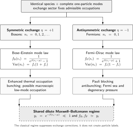
Exchange symmetry fixes the admissible occupations. Equilibrium weighting then gives Bose–Einstein or Fermi–Dirac mode laws. Both approach the same Maxwell–Boltzmann law when every mode activity $y_i=e^{-\beta(\epsilon_i-\mu)}$ is small; that shared limit does not erase the underlying exchange sector.

The arrows in the figure are one-way implications under stated assumptions. Observing a nearly Maxwell–Boltzmann distribution does not mean that the particles have become distinguishable. It means that exchange corrections are too small to matter for the observables and accuracy under consideration.

Complete Single-Particle Modes

The index $i$ must contain every quantum number needed to distinguish orthogonal one-particle states. Depending on the system, it may mean

$$i = (\mathbf k,\sigma,a,\nu,\ldots),$$

where $\mathbf k$ is momentum, $\sigma$ is spin or polarization, $a$ is a band or species label, and $\nu$ is a trap level.

This completeness is crucial for the Pauli principle. Two fermions may have the same spatial wavefunction or the same energy if another mode label differs. For example, an orbital in a spin-independent electron model can hold two electrons because

$$(\phi,\uparrow) \neq (\phi,\downarrow).$$

What is forbidden is double occupation of the same spin-orbital:

$$n_{\phi,\sigma} \in \{0,1\}.$$

Similarly, a degeneracy $g$ does not multiply the occupation of one mode. It means that there are $g$ distinct modes at the same energy. If each has mean occupation $f(\epsilon)$, the mean occupation of the whole level is

$$\overline N_{\epsilon} = g f(\epsilon).$$

The occupation-number representation develops this bookkeeping systematically.

Exchange Sectors

Bosons

Bosonic many-particle states are symmetric under exchange. In an occupation basis, every complete mode permits

$$n_i = 0,1,2,\ldots.$$

Integer-spin elementary particles are bosons, as are many composite objects in an appropriate low-energy regime. Photons, phonons, magnons, helium-4 atoms, and integer-spin ultracold atoms are common examples, although the meaning and conservation of particle number differ among them.

Unrestricted mode occupation makes macroscopic occupation possible, but it does not by itself guarantee Bose–Einstein condensation. Condensation also depends on the spectrum, dimensionality, geometry, particle-number constraint, and thermodynamic limit.

Fermions

Fermionic many-particle states are antisymmetric under exchange. The occupation of a complete mode is restricted to

$$n_i = 0,1.$$

This is the occupation-number form of Pauli exclusion. Electrons, protons, neutrons, quarks, helium-3 atoms, and many half-integer-spin atomic isotopes are fermions in their relevant regimes.

Exclusion is kinematic. It operates even for an ideal gas and produces a filled Fermi sea, degeneracy pressure, and Pauli blocking without requiring a repulsive potential.

Spin and statistics

In nonrelativistic many-body theory, a species’ exchange sector is normally part of the model specification. Relativistic quantum field theory explains the observed pairing through the spin–statistics theorem: under assumptions including Lorentz invariance, locality, positive energy, and a positive-definite state space, integer-spin fields have bosonic statistics and half-integer-spin fields have fermionic statistics.

The spin–statistics preview states that result and its assumptions. It should not be replaced by the mnemonic “integer means boson, half-integer means fermion” when discussing effective excitations or lower-dimensional systems.

Dimensional caveat

In three spatial dimensions, ordinary pointlike identical particles lead to the bosonic and fermionic alternatives above. In two spatial dimensions, exchanges are described by braid topology and richer anyonic statistics can occur. The Bose/Fermi overview here is therefore not a classification of every possible topological quasiparticle.

Ideal-Mode Thermodynamics

For independent modes, the grand Hamiltonian factorizes:

$$K = H-\mu N = \sum_i (\epsilon_i-\mu)n_i.$$

Introduce the fugacity and one-mode activity

$$z = e^{\beta\mu}, \qquad y_i = z e^{-\beta\epsilon_i} = e^{-\beta(\epsilon_i-\mu)}.$$

The activity $y_i$ is invariant under a simultaneous energy-zero shift

$$\epsilon_i \mapsto \epsilon_i+C, \qquad \mu \mapsto \mu+C.$$

Only $\epsilon_i-\mu$ is physically relevant in the occupation law.

One-mode partition sums

For a bosonic mode,

$$\xi_i^{\mathrm B} = \sum_{n=0}^{\infty} y_i^n = \frac{1}{1-y_i}, \qquad y_i<1.$$

For a fermionic mode,

$$\xi_i^{\mathrm F} = \sum_{n=0}^{1} y_i^n = 1+y_i.$$

The full grand partition function is

$$\Xi = \prod_i \xi_i.$$

This product is the source of grand-canonical mode independence. The neighboring Bose–Einstein and Fermi–Dirac pages derive all moments and limiting forms explicitly.

Unified notation

With

$$\eta = \begin{cases} +1, & \text{bosons},\\ -1, & \text{fermions}, \end{cases}$$

the two one-mode factors can be written as

$$\xi_i = (1-\eta y_i)^{-\eta}.$$

The logarithm of the grand partition function and the grand potential are

$$\ln\Xi = -\eta \sum_i \ln(1-\eta y_i),$$ $$\Omega = -k_{\mathrm B}T\ln\Xi = \eta k_{\mathrm B}T \sum_i \ln(1-\eta y_i).$$

A logarithmic derivative gives the mean occupation

$$f_{\eta}(\epsilon_i) \equiv \overline n_i = y_i \frac{\partial\ln\xi_i}{\partial y_i} = \frac{y_i}{1-\eta y_i}.$$

Equivalently,

$$f_{\eta}(\epsilon) = \frac{1}{e^{\beta(\epsilon-\mu)}-\eta}.$$

The variance is

$$\operatorname{Var}(n_i) = y_i \frac{\partial\overline n_i}{\partial y_i} = f_i(1+\eta f_i).$$

Thus

$$\begin{aligned} \operatorname{Var}_{\mathrm B}(n_i) &= f_i(1+f_i), \\ \operatorname{Var}_{\mathrm F}(n_i) &= f_i(1-f_i). \end{aligned}$$

The opposite signs are a compact signature of Bose enhancement and Pauli blocking in ideal thermal modes.

Comparison table

Feature	Bose–Einstein	Fermi–Dirac	Maxwell–Boltzmann regime
Exchange sector	symmetric	antisymmetric	underlying sector remains Bose or Fermi
Allowed ideal-mode occupation	$0,1,2,\ldots$	$0,1$	many-particle exchange cycles negligible
One-mode grand factor	$(1-y_i)^{-1}$	$1+y_i$	$e^{y_i}$ in the Poisson ideal-gas description
Mean occupation	$(e^{\beta(\epsilon_i-\mu)}-1)^{-1}$	$(e^{\beta(\epsilon_i-\mu)}+1)^{-1}$	$e^{-\beta(\epsilon_i-\mu)}$
Ideal-mode variance	$f_i(1+f_i)$	$f_i(1-f_i)$	$f_i$
Number constraint	$\mu<\epsilon_0$ for a finite ideal spectrum	no analogous convergence bound	fugacity fixed by density
Qualitative effect	enhanced occupation and bunching in thermal fields	suppressed occupation fluctuations and antibunching	approximately independent dilute particles
Characteristic low-temperature structure	possible macroscopic low-mode occupation	Fermi sea and a thermally active shell	classical law eventually fails at fixed density

The Maxwell–Boltzmann column describes a limiting regime, not a third exchange eigenvalue $\eta=0$. Setting $\eta=0$ is a useful algebraic shorthand for the leading dilute term, but it should not be interpreted as a new quantum exchange sector.

Probability Laws of One Ideal Mode

The mean occupation does not contain all statistical information. The full one-mode law clarifies the differences.

For bosons,

$$p_i^{\mathrm B}(n) = (1-y_i)y_i^n, \qquad n = 0,1,2,\ldots.$$

This geometric distribution has a long occupation tail when $y_i$ approaches one.

For fermions,

$$p_i^{\mathrm F}(0) = \frac{1}{1+y_i}, \qquad p_i^{\mathrm F}(1) = \frac{y_i}{1+y_i}.$$

It is a Bernoulli distribution because no higher occupation is allowed.

In the dilute classical grand-canonical description,

$$p_i^{\mathrm{MB}}(n) = e^{-y_i} \frac{y_i^n}{n!}, \qquad n = 0,1,2,\ldots,$$

which is Poissonian with mean and variance $y_i$. These mode distributions are ensemble statements; they should not be confused with the spatial distribution of particle positions or with arbitrary detector-count distributions.

The Maxwell–Boltzmann Regime

A shared asymptotic law

When

$$y_i = e^{-\beta(\epsilon_i-\mu)} \ll 1$$

for all appreciably occupied modes,

$$f_{\eta} = \frac{y_i}{1-\eta y_i} = y_i + \eta y_i^2 + O(y_i^3).$$

The leading term is independent of $\eta$:

$$f_{\mathrm{MB}}(\epsilon_i) = z e^{-\beta\epsilon_i}.$$

The first correction is positive for bosons and negative for fermions. Consequently, at fixed $z$ and $T$, a bosonic mode is slightly more occupied and a fermionic mode slightly less occupied than its Maxwell–Boltzmann approximation.

Phase-space criterion

For a uniform nonrelativistic gas in $d$ dimensions, define the thermal wavelength

$$\lambda_T = \sqrt{ \frac{2\pi\hbar^2}{m k_{\mathrm B}T} }.$$

If $g$ is the internal degeneracy, a useful phase-space-density parameter is

$$\mathcal D = \frac{n\lambda_T^d}{g}.$$

The Maxwell–Boltzmann regime requires

$$\mathcal D \ll 1.$$

This condition says that the mean occupation of a thermal phase-space cell is small. It is more informative than “high temperature” alone: increasing density or reducing mass can make exchange effects important even when the absolute temperature seems large.

For a three-dimensional ideal gas in the dilute regime,

$$\mathcal D \simeq z.$$

Precise higher-order relations and the leading Bose/Fermi virial corrections are derived on Classical Limit of Quantum Statistics.

Distinguishable labels are approximate bookkeeping

Classical calculations often assign temporary labels to particles and divide the state count by $N!$. This works because exchange-related wave-packet overlaps are negligible in the dilute regime. The exact quantum particles do not acquire observable identities. Their bosonic or fermionic sector remains intact, while permutation cycles beyond the identity contribute negligibly to coarse thermodynamic quantities.

From Occupations to Thermodynamics

Once $f_i$ is known, additive one-body observables reduce to mode sums. For ideal particles,

$$\overline N = \sum_i f_i,$$ $$U = \sum_i \epsilon_i f_i.$$

If an observable is diagonal in the same one-particle basis,

$$A = \sum_i a_i n_i,$$

then

$$\langle A\rangle = \sum_i a_i f_i.$$

The distribution therefore acts as a weighting function. It does not supply the spectrum or density of states; those belong to the Hamiltonian and geometry.

Density-of-states form

For a dense spectrum, replace the sum by

$$\sum_i F(\epsilon_i) \longrightarrow \int d\epsilon\, g(\epsilon)F(\epsilon),$$

where $g(\epsilon)$ counts complete one-particle modes per unit energy. Then

$$N = \int d\epsilon\, g(\epsilon)f_{\eta}(\epsilon),$$ $$U = \int d\epsilon\, g(\epsilon)\epsilon f_{\eta}(\epsilon).$$

For bosons near condensation, the lowest mode may need to be separated explicitly:

$$N = N_0 + \int_{\epsilon>\epsilon_0} d\epsilon\, g_{\mathrm{ex}}(\epsilon) f_{\mathrm B}(\epsilon).$$

Whether the excited-state integral has a finite capacity determines whether a conventional condensation transition is possible in the thermodynamic limit.

Pressure and the grand potential

For a homogeneous system,

$$P = - \left( \frac{\partial\Omega}{\partial V} \right)_{T,\mu}.$$

If $\Omega$ is extensive and boundary effects are negligible,

$$\Omega = -PV.$$

Different occupation laws change $\Omega$ and therefore the equation of state. In the dilute regime, the first exchange correction lowers the ideal Bose-gas pressure and raises the ideal Fermi-gas pressure at fixed $N$, $V$, and $T$.

Entropy per mode

For independent ideal modes, the entropy can be expressed directly through $f_i$. Unified notation gives

$$\frac{s_i}{k_{\mathrm B}} = \eta(1+\eta f_i) \ln(1+\eta f_i) - f_i\ln f_i.$$

For bosons this becomes

$$\frac{s_i^{\mathrm B}}{k_{\mathrm B}} = (1+f_i)\ln(1+f_i) - f_i\ln f_i,$$

whereas for fermions

$$\frac{s_i^{\mathrm F}}{k_{\mathrm B}} = -f_i\ln f_i - (1-f_i)\ln(1-f_i).$$

The total ideal-mode entropy is $S=\sum_i s_i$. The entropy page develops the density-operator definition and thermodynamic relations.

Chemical Potential and Number Conservation

The chemical potential is not a universal property of “being a boson” or “being a fermion.” It appears when an ensemble constrains the mean value of a conserved or effectively conserved number.

Bosonic convergence bound

For a finite ideal bosonic spectrum with lowest energy $\epsilon_0$, convergence of the ground-mode geometric series requires

$$\mu < \epsilon_0.$$

The ground-mode occupation is

$$N_0 = \frac{1}{e^{\beta(\epsilon_0-\mu)}-1}.$$

As $\mu$ approaches $\epsilon_0$ from below, $N_0$ grows. In a thermodynamic-limit treatment of a condensed phase one often writes $\mu\to\epsilon_0$, while treating the macroscopically occupied mode separately. Substituting $\mu=\epsilon_0$ blindly into the one-mode geometric sum creates a divergence rather than a normalized finite-system probability distribution.

Fermionic chemical potential

For a fermionic mode,

$$\xi_i^{\mathrm F} = 1+e^{-\beta(\epsilon_i-\mu)}$$

is finite for every finite $\mu$. There is no boson-like convergence bound $\mu<\epsilon_0$. At low temperature and fixed density, $\mu$ approaches the Fermi energy of the ideal gas, with corrections determined by the density of states.

Nonconserved quasiparticles

Photons and phonons in ordinary thermal equilibrium can be created and destroyed by the material environment. Their equilibrium chemical potential is therefore

$$\mu = 0.$$

The same statement often applies to magnons and other quasiparticles, but pumping or approximate number conservation can produce an effective nonzero chemical potential over a restricted time window. The assumptions and equilibration processes must be stated.

The chemical-potential page treats these distinctions in detail.

Bosonic Consequences

The Bose denominator produces several related but distinct phenomena.

Enhanced occupation

At fixed activity $y$,

$$f_{\mathrm B} = \frac{y}{1-y} > y.$$

Relative to the dilute law, already occupied low-energy modes receive enhanced statistical weight. In transition-rate language this often appears through factors $1+n$, but that kinetic statement requires a dynamical calculation and should not be inferred from equilibrium occupations alone.

Super-Poissonian thermal mode fluctuations

An ideal thermal bosonic mode satisfies

$$\operatorname{Var}(n) = f(1+f) > f.$$

This excess variance underlies thermal bunching in suitable coherence measurements. It is not a universal statement about all bosonic states: coherent states have Poissonian number fluctuations, and number states have zero number variance.

Possible macroscopic occupation

When a conserved boson density exceeds the capacity of the excited states, the excess particles occupy the lowest mode macroscopically. The occurrence and character of this phenomenon depend on the density of states and thermodynamic limit. The full three-dimensional uniform-gas thermodynamics belongs to Ideal Bose Gas.

No implied attraction

Bosonic enhancement is sometimes described as an “effective attraction.” That phrase can be useful for the sign of a virial correction, but it is not a microscopic force. An ideal Bose gas has no interparticle potential, and interacting bosons can have repulsive, attractive, or more complicated interactions.

Fermionic Consequences

Pauli blocking

At fixed activity $y$,

$$f_{\mathrm F} = \frac{y}{1+y} < y.$$

The occupation of a mode is suppressed relative to the dilute law because the state cannot hold a second identical fermion. In scattering kinetics, the availability of a final fermionic mode is represented by a factor $1-f$.

Sub-Poissonian ideal-mode fluctuations

For a thermal fermionic mode,

$$\operatorname{Var}(n) = f(1-f) < f.$$

The variance vanishes when $f$ approaches either zero or one. A nearly filled mode is quiet because both additional occupation and vacancy fluctuations are rare.

Fermi sea and active shell

At zero temperature,

$$\lim_{T\to0} f_{\mathrm F}(\epsilon) = \Theta(\mu-\epsilon)$$

away from $\epsilon=\mu$. Modes below the Fermi energy are filled and those above are empty. At small nonzero temperature, only an energy shell of width roughly $k_{\mathrm B}T$ around the chemical potential changes appreciably. This active shell controls the low-temperature heat capacity and many transport coefficients.

Degeneracy pressure

Filling successively higher momentum states costs kinetic energy even without interactions. The associated volume dependence of the ground-state energy produces fermion degeneracy pressure. It is a consequence of antisymmetry and the spectrum, not an electrostatic repulsion.

The uniform-gas formulas are developed on Ideal Fermi Gas.

Grand-Canonical Independence and Canonical Correlations

For an ideal grand-canonical gas, the density operator factorizes over modes:

$$\rho_{\mathrm{GC}} = \bigotimes_i \rho_i.$$

Consequently, distinct ideal modes are statistically independent:

$$\operatorname{Cov}(n_i,n_j) = 0, \qquad i\neq j.$$

This does not remain exactly true in the canonical ensemble. If the total number is fixed,

$$\sum_i n_i = N$$

in every microstate. Therefore

$$\operatorname{Var} \left( \sum_i n_i \right) = 0.$$

Expanding the variance gives

$$\sum_i \operatorname{Var}(n_i) + 2\sum_{i<j} \operatorname{Cov}(n_i,n_j) = 0.$$

The off-diagonal covariances must cancel the positive diagonal variances. Thus the familiar one-mode fluctuation formulas are not exact canonical formulas at finite $N$.

For local thermodynamic observables, canonical and grand-canonical predictions often agree in a regular thermodynamic limit. Global number fluctuations, condensate fluctuations, and finite systems can retain important ensemble dependence. The ensemble-equivalence page states the conditions and exceptions.

Internal Degeneracy and Mixtures

Suppose a translational mode $\mathbf k$ has $g$ internal states $a=1,\ldots,g$ with equal energy. Then

$$N = \sum_{\mathbf k} \sum_{a=1}^{g} f(\epsilon_{\mathbf k}).$$

The degeneracy contributes a factor $g$:

$$N = g \sum_{\mathbf k} f(\epsilon_{\mathbf k}).$$

For fermions, each complete mode $(\mathbf k,a)$ still has occupation zero or one. A factor $g=2$ for spin does not weaken exclusion; it counts two orthogonal spin modes.

For a mixture of species $s$, use separate chemical potentials when the corresponding particle numbers are independently conserved:

$$f_s(\epsilon) = \frac{1}{ e^{\beta(\epsilon-\mu_s)}-\eta_s }.$$

Chemical reactions or conversion processes impose relations among the $\mu_s$. A mixture can contain both bosonic and fermionic species, and exchange symmetry applies only within each set of identical particles.

Temperature and Density Regimes

The relevant control parameter is not temperature alone. Density, mass, degeneracy, dimensionality, and dispersion all matter.

Dilute classical regime

When

$$\mathcal D = \frac{n\lambda_T^d}{g} \ll 1,$$

exchange corrections are small and Maxwell–Boltzmann statistics is accurate. Typical occupation numbers are much less than one.

Bose-degenerate regime

For conserved bosons, increasing $\mathcal D$ drives $\mu$ toward the lowest one-particle energy. Low-energy occupations become large, and the continuum excited states may saturate. Whether a sharp transition occurs depends on the low-energy density of states and the thermodynamic limit.

Fermi-degenerate regime

For fermions, degeneracy becomes important when the temperature is comparable to or below the Fermi temperature:

$$T \lesssim T_{\mathrm F}, \qquad k_{\mathrm B}T_{\mathrm F} = \epsilon_{\mathrm F}.$$

Most low-energy modes are then nearly filled. The small parameter for low-temperature expansions is usually $T/T_{\mathrm F}$, not the fugacity.

Zero-temperature limits

At fixed nonzero density, the zero-temperature limit is strongly quantum:

• ideal fermions fill a Fermi sea;
• conserved ideal bosons occupy the lowest available mode macroscopically under the usual condensation conditions;
• Maxwell–Boltzmann statistics is not a valid fixed-density $T\to0$ limit.

The phrase “classical ground state” therefore cannot be obtained by simply lowering $T$ in a Maxwell–Boltzmann gas.

Dimensionality, Traps, and Dispersions

The one-mode factor depends only on $\beta(\epsilon_i-\mu)$, but macroscopic thermodynamics depends on how many modes occur at each energy.

For an isotropic continuum with dispersion

$$\epsilon(\mathbf p) \propto p^s$$

in $d$ dimensions, the low-energy density of states scales as

$$g(\epsilon) \propto \epsilon^{d/s-1}.$$

This exponent controls infrared convergence for bosons and the relation among density, Fermi momentum, and Fermi energy for fermions.

In a harmonic trap, the level counting differs from that of a box. On a lattice, the spectrum has a finite band and may contain van Hove singularities. In relativistic systems, both dispersion and antiparticle sectors change. These differences alter thermodynamic integrals while leaving the local ideal-mode Bose or Fermi factor unchanged.

A finite spectrum also smooths thermodynamic singularities. Sharp phase transitions require an appropriate thermodynamic limit; a finite trapped cloud exhibits crossovers and finite-size shifts.

Interactions and Quasiparticles

Exchange statistics survives interactions, but the elementary ideal-gas occupation formulas need not.

For an interacting Hamiltonian,

$$H \neq \sum_i \epsilon_i n_i,$$

the bare mode occupations generally do not factorize. The exact equilibrium density operator remains

$$\rho \propto e^{-\beta(H-\mu N)},$$

but

$$\langle n_i\rangle \neq \frac{1}{e^{\beta(\epsilon_i-\mu)}-\eta}$$

for arbitrary choices of bare $\epsilon_i$.

Several controlled possibilities remain:

• a quadratic Hamiltonian may be diagonalized exactly into independent normal modes;
• weakly interacting systems may admit long-lived quasiparticles;
• mean-field theory may produce effective single-particle energies and self-consistency equations;
• spectral-function methods distribute occupation over both energy and momentum;
• strongly correlated systems may have no useful particle-like mode description.

Even when quasiparticles obey a Bose or Fermi distribution in energy, the measured bare-particle momentum distribution can include coherence factors and incoherent spectral weight. Calling every observed curve “Bose–Einstein” or “Fermi–Dirac” can therefore hide the actual observable being modeled.

Equilibrium and Nonequilibrium

The equilibrium laws require a temperature and chemical potentials that consistently describe the relevant degrees of freedom. They can fail or require modification when:

• the system is driven or rapidly expanding;
• relaxation among modes is too slow;
• several subsystems have different effective temperatures;
• particle number is only approximately conserved;
• integrability preserves additional charges;
• the state is many-body localized or prethermal;
• gain and loss balance in an open quantum system.

A fitted curve of the form

$$\frac{1}{e^{\beta_{\mathrm{eff}}(\epsilon-\mu_{\mathrm{eff}})}-\eta}$$

is evidence for an effective description over the fitted range, not proof of global thermal equilibrium. One should test other observables and conserved quantities.

Experimental Signatures

Quantum statistics is inferred through a web of observables rather than a single denominator sign.

Momentum and energy distributions

Time-of-flight imaging in ultracold gases, photoemission in solids, and spectroscopic probes can reveal occupied states. Interpreting the signal requires matrix elements, detector response, interactions, and often a spectral function.

Noise and correlation measurements

Second-order correlations can show bunching for thermal bosons and antibunching for identical fermions in the same internal state. The relevant observable is usually a normal-ordered field correlation, not simply the variance of a globally integrated particle number.

Thermodynamic equations of state

Pressure, compressibility, entropy, and heat capacity distinguish classical and quantum-degenerate regimes. Fermion degeneracy pressure and the bosonic saturation of excited states are bulk consequences of mode counting.

Transport and scattering

Final-state factors $1+f$ for bosons and $1-f$ for fermions modify kinetic rates. These factors encode availability and stimulation in a many-body background; a complete rate also contains matrix elements, conservation laws, and the occupations of all incoming and outgoing modes.

Worked Mini-Examples

One bosonic oscillator mode

For a mode of energy $\epsilon=\hbar\omega$ whose number is not conserved, set $\mu=0$. Then

$$f_{\mathrm B} = \frac{1}{e^{\beta\hbar\omega}-1}.$$

At high temperature,

$$k_{\mathrm B}T \gg \hbar\omega,$$

the occupation is

$$f_{\mathrm B} \simeq \frac{k_{\mathrm B}T}{\hbar\omega}.$$

At low temperature it is exponentially small:

$$f_{\mathrm B} \simeq e^{-\beta\hbar\omega}.$$

The first limit is classical equipartition for the mode; the second reflects a quantum excitation gap.

A spin-degenerate fermionic level

Take one spatial orbital of energy $\epsilon$ with two spin states. There are two complete modes, $(\phi,\uparrow)$ and $(\phi,\downarrow)$. Their mean total occupation is

$$\overline N_{\epsilon} = 2 \frac{1}{e^{\beta(\epsilon-\mu)}+1}.$$

The level may contain zero, one, or two electrons, but no spin-orbital may contain two. As $T\to0$, the level is doubly occupied if $\epsilon<\mu$ and empty if $\epsilon>\mu$.

Comparing equal activity

Let a mode have activity

$$y = 0.1.$$

Then

$$f_{\mathrm B} = \frac{0.1}{0.9} \simeq 0.111,$$ $$f_{\mathrm{MB}} = 0.100,$$ $$f_{\mathrm F} = \frac{0.1}{1.1} \simeq 0.0909.$$

The dilute approximation is already accurate at roughly the ten-percent level for this mode. The opposite deviations display the leading exchange correction without invoking any interaction potential.

A Decision Workflow

When choosing a statistical description, proceed in this order.

1. Identify the species. Determine which particles or quasiparticles are identical and whether conversions occur.
2. Specify the exchange sector. State whether each species is bosonic or fermionic; note any lower-dimensional topological exception.
3. Define complete modes. Include momentum, spin, band, polarization, trap, and species labels as needed.
4. Choose the ensemble. Decide which energy, particle numbers, and other charges are fixed or controlled on average.
5. Check the Hamiltonian. Verify whether it factorizes into independent modes or requires an interacting treatment.
6. Determine the regime. Estimate fugacity, phase-space density, $T/T_{\mathrm F}$, and proximity to a bosonic ground-state boundary.
7. Insert the density of states. Translate mode occupations into the observable appropriate to the geometry and dispersion.
8. Test limits and normalization. Check dilute, zero-temperature, high-temperature, and finite-size behavior.

This workflow prevents a common inversion: selecting a familiar distribution first and only later asking whether its assumptions match the system.

Common Mistakes

Treating Maxwell–Boltzmann statistics as a third quantum exchange sector

Maxwell–Boltzmann statistics is the leading dilute behavior of either bosons or fermions. The particles remain identical, and sufficiently precise exchange-sensitive measurements can still distinguish the sectors.

Saying that all bosons occupy the same state

Bosons may share a mode. At finite temperature, an ideal Bose gas generally occupies many modes. Macroscopic ground-mode occupation requires additional thermodynamic conditions.

Saying that fermions cannot have the same energy

Pauli exclusion forbids the same complete one-particle mode, not the same energy. Degenerate orthogonal modes can all be occupied.

Forgetting internal degeneracy

Spin, polarization, valley, flavor, or band labels change the number of modes. Omitting a degeneracy factor changes density and thermodynamic scales.

Using the Bose formula at the convergence boundary in a finite system

For a finite ideal bosonic mode, $\mu=\epsilon_0$ makes the geometric sum non-normalizable. Separate the condensate mode and take the thermodynamic limit with care.

Applying ideal-mode occupations to an interacting bare spectrum

Interactions do not change bosons into fermions or vice versa, but they can invalidate factorization and redistribute spectral weight. A Bose or Fermi denominator is not a substitute for solving the interacting model.

Confusing bunching with bosonic identity

Thermal bosons bunch under appropriate measurements, but coherent bosonic fields can be Poissonian and number states can be antibunched. Exchange sector, quantum state, and measured correlation must all be specified.

Ignoring ensemble dependence of fluctuations

Grand-canonical ideal-mode variances need not equal canonical finite-system variances. Mean local thermodynamics can agree while global fluctuations differ.

Assuming low temperature always means quantum degeneracy

Degeneracy is controlled by dimensionless ratios such as $n\lambda_T^d/g$ or $T/T_{\mathrm F}$. A very dilute heavy gas can remain classical at a temperature that is “low” in everyday units.

Exercises

Unified mode factor

Starting from

$$\xi(y) = (1-\eta y)^{-\eta},$$

derive the mean occupation and variance using derivatives with respect to $y$. Verify both signs $\eta=\pm1$.

Solution

The logarithm is

$$\ln\xi = -\eta\ln(1-\eta y).$$

Since $\eta^2=1$,

$$\frac{\partial\ln\xi}{\partial y} = \frac{1}{1-\eta y}.$$

Therefore

$$f = y \frac{\partial\ln\xi}{\partial y} = \frac{y}{1-\eta y}.$$

For a grand-canonical mode,

$$\operatorname{Var}(n) = y \frac{\partial f}{\partial y}.$$

Differentiating gives

$$\operatorname{Var}(n) = \frac{y}{(1-\eta y)^2}.$$

Because

$$1+\eta f = \frac{1}{1-\eta y},$$

this is

$$\operatorname{Var}(n) = f(1+\eta f).$$

For $\eta=+1$, one obtains the Bose geometric factor, $f=y/(1-y)$, and variance $f(1+f)$. For $\eta=-1$, one obtains the Fermi factor, $f=y/(1+y)$, and variance $f(1-f)$.

Leading dilute correction

Expand the Bose and Fermi occupations through order $y^2$. At fixed activity, which distribution lies above the Maxwell–Boltzmann value?

Solution

For $|y|<1$,

$$\frac{y}{1-\eta y} = y + \eta y^2 + O(y^3).$$

Thus

$$f_{\mathrm B} = y+y^2+O(y^3),$$ $$f_{\mathrm F} = y-y^2+O(y^3).$$

The Maxwell–Boltzmann value is $f_{\mathrm{MB}}=y$. Hence the Bose occupation lies above it and the Fermi occupation lies below it at fixed $y$. This comparison holds at fixed activity; comparisons at fixed density require adjusting $\mu$ and can change the wording of the thermodynamic effect.

Complete mode labels

A spatial orbital of energy $\epsilon$ is sixfold degenerate because of spin and valley labels: $\sigma=\uparrow,\downarrow$ and $v=1,2,3$. How many identical fermions can occupy the energy level? What is its mean occupation in grand-canonical equilibrium?

Solution

The complete modes are

$$i = (\phi,\sigma,v).$$

There are

$$g = 2\times3 = 6$$

orthogonal modes. Each can contain at most one identical fermion, so the level can contain at most six.

Every mode has mean occupation

$$f_{\mathrm F}(\epsilon) = \frac{1}{e^{\beta(\epsilon-\mu)}+1}.$$

Therefore

$$\overline N_{\epsilon} = 6 f_{\mathrm F}(\epsilon).$$

The exclusion principle is obeyed mode by mode; degeneracy supplies more modes rather than allowing multiple occupancy of one mode.

Canonical anticorrelations

Two modes contain a fixed total of one particle, so $n_1+n_2=1$ in every microstate. Show that their covariance is negative and express it in terms of $p=\langle n_1\rangle$.

Solution

Because $n_2=1-n_1$,

$$\langle n_2\rangle = 1-p.$$

Also, $n_1n_2=0$ in every allowed microstate. Hence

$$\operatorname{Cov}(n_1,n_2) = \langle n_1n_2\rangle - \langle n_1\rangle \langle n_2\rangle$$

becomes

$$\operatorname{Cov}(n_1,n_2) = -p(1-p).$$

The variance of either Bernoulli occupation is $p(1-p)$, so

$$\operatorname{Var}(n_1+n_2) = p(1-p) + p(1-p) - 2p(1-p) = 0.$$

The negative covariance arises from the fixed-number constraint, independently of whether the single particle is called bosonic or fermionic.

Bosonic ground-mode boundary

Let $\delta=\epsilon_0-\mu>0$. Find the leading behavior of the bosonic ground-mode occupation for $\beta\delta\ll1$. Explain why setting $\delta=0$ is not a normalized finite-mode grand-canonical state.

Solution

The occupation is

$$N_0 = \frac{1}{e^{\beta\delta}-1}.$$

For $\beta\delta\ll1$,

$$e^{\beta\delta}-1 = \beta\delta + O((\beta\delta)^2),$$

so

$$N_0 \simeq \frac{1}{\beta\delta}.$$

At $\delta=0$, the one-mode activity is $y_0=1$ and

$$\xi_0 = \sum_{n=0}^{\infty}1$$

diverges. There is no normalized geometric probability distribution for that finite mode. Condensed-phase thermodynamics instead separates the macroscopic mode and takes a controlled thermodynamic limit.

Zero-temperature Fermi step

Evaluate

$$\lim_{\beta\to\infty} \frac{1}{e^{\beta(\epsilon-\mu)}+1}$$

for $\epsilon<\mu$ and $\epsilon>\mu$. What is the value exactly at $\epsilon=\mu$ for finite $T$?

Solution

If $\epsilon<\mu$, then

$$\beta(\epsilon-\mu) \longrightarrow -\infty,$$

so the exponential vanishes and

$$f_{\mathrm F} \longrightarrow 1.$$

If $\epsilon>\mu$, the exponential diverges and

$$f_{\mathrm F} \longrightarrow 0.$$

At $\epsilon=\mu$ and any finite $T$,

$$f_{\mathrm F}(\mu) = \frac{1}{2}.$$

The value at a single energy does not affect continuum thermodynamic integrals. At zero temperature the distribution is represented by the step function $\Theta(\mu-\epsilon)$ up to that conventional boundary value.

Exchange sector versus observed number variance

Classify the following statements as valid or invalid, and explain: (a) every bosonic state has $\operatorname{Var}(n)>\langle n\rangle$; (b) a Poissonian count distribution proves that particles are distinguishable; (c) a thermal ideal fermionic mode has sub-Poissonian occupation fluctuations.

Solution

(a) is invalid. The formula

$$\operatorname{Var}(n) = f(1+f)$$

describes a thermal ideal bosonic mode. A coherent state has $\operatorname{Var}(n)=\langle n\rangle$, while a number state has zero number variance.

(b) is invalid. Bosonic coherent states are Poissonian, and dilute bosons or fermions approach Poissonian Maxwell–Boltzmann mode statistics. Exchange identity is not erased by a Poissonian observation.

(c) is valid under its stated assumptions because

$$\operatorname{Var}(n) = f(1-f) \leq f.$$

The qualification “thermal ideal mode” matters; other observables, mode groupings, and ensemble constraints can have different counting statistics.

Cross-Links

• Quantum Gas Formula Sheet
• Symmetrization Postulate
• Symmetric and Antisymmetric Wavefunctions
• Occupation-Number Representation
• Grand-Canonical Ensemble
• Partition Functions
• Chemical Potential
• Maxwell–Boltzmann Limit
• Bose–Einstein Statistics
• Fermi–Dirac Statistics
• Ideal Bose Gas
• Ideal Fermi Gas
• Classical Limit of Quantum Statistics
• Thermodynamic Limit
• Ensemble Equivalence
• Ensemble Formula Sheet
• Historical Development of Identical-Particle Statistics

References

• S. N. Bose, “Plancks Gesetz und Lichtquantenhypothese,” Zeitschrift für Physik 26, 178–181 (1924), doi:10.1007/BF01327326.
• A. Einstein, “Quantentheorie des einatomigen idealen Gases,” Sitzungsberichte der Preußischen Akademie der Wissenschaften, Physikalisch-mathematische Klasse, 261–267 (1924); “Zweite Abhandlung,” 3–14 (1925).
• E. Fermi, “Zur Quantelung des idealen einatomigen Gases,” Zeitschrift für Physik 36, 902–912 (1926), doi:10.1007/BF01400221.
• P. A. M. Dirac, “On the Theory of Quantum Mechanics,” Proceedings of the Royal Society A 112, 661–677 (1926), doi:10.1098/rspa.1926.0133.
• R. K. Pathria and P. D. Beale, Statistical Mechanics, 3rd ed., Elsevier (2011).
• K. Huang, Statistical Mechanics, 2nd ed., Wiley (1987).
• M. Kardar, Statistical Physics of Particles, Cambridge University Press (2007).
• L. D. Landau and E. M. Lifshitz, Statistical Physics, Part 1, 3rd ed., Butterworth–Heinemann (1980).
• A. L. Fetter and J. D. Walecka, Quantum Theory of Many-Particle Systems, Dover (2003).
• C. J. Pethick and H. Smith, Bose–Einstein Condensation in Dilute Gases, 2nd ed., Cambridge University Press (2008).
• N. W. Ashcroft and N. D. Mermin, Solid State Physics, Brooks/Cole (1976).