Anderson Impurity Model

One-Sentence Description

The single-impurity Anderson model couples one interacting spinful fermion orbital to a noninteracting bath, retaining the impurity’s empty, singly occupied, and doubly occupied charge sectors while hybridization makes local charge fluctuate coherently.

Canonical Scope

This dossier is the canonical home for:

• a compact, convention-complete specification of the single-orbital Anderson impurity model;
• the distinction between bath density of states and hybridization function;
• its Hilbert space, symmetries, charge regimes, control parameters, and model boundaries;
• a precise map of analytic limits, integrable formulations, and controlled numerical methods;
• an observable–method dictionary;
• an exact two-orbital finite-bath benchmark.

Anderson Impurity Model Preview owns the detailed teaching treatment of atomic thermodynamics, the resonant-level Green function, correlated spectral anatomy, the Friedel sum rule, quantum-dot interpretation, impurity thermodynamics, and the DMFT loop. Effective Hamiltonians in Many-Body Systems owns the comparative virtual-charge derivation of Kondo exchange, while the Kondo Model dossier owns the resulting spin-only model.

Common Many-Body Hamiltonians remains the compact formula sheet. The purpose here is to say exactly what must be specified, what each limit controls, and what a finite implementation must reproduce.

The baseline is one spin-degenerate interacting orbital, one equilibrium fermionic bath, spin-independent hybridization, repulsive $U$, no magnetic field, and all one-particle energies measured relative to the chemical potential. Departures from that baseline are labeled explicitly.

Model Definition

Write the Hamiltonian as

$$H_{\mathrm A} = H_{\mathrm{bath}} + H_d + H_{\mathrm{hyb}}.$$

The bath is quadratic,

$$H_{\mathrm{bath}} = \sum_{k,\sigma} \epsilon_k c_{k\sigma}^\dagger c_{k\sigma}.$$

The impurity contains one spinful orbital,

$$H_d = \epsilon_d \sum_\sigma n_{d\sigma} + U n_{d\uparrow}n_{d\downarrow},$$

where

$$n_{d\sigma} = d_\sigma^\dagger d_\sigma.$$

Coherent bath–impurity transfer is

$$H_{\mathrm{hyb}} = \sum_{k,\sigma} \left( V_k c_{k\sigma}^\dagger d_\sigma + V_k^*d_\sigma^\dagger c_{k\sigma} \right).$$

Hermiticity requires both terms. A phase convention may move phases between $V_k$, bath orbitals, and $d_\sigma$, but physical hybridization data are unchanged.

Chemical-potential convention

The displayed $\epsilon_k$ and $\epsilon_d$ are energies relative to the equilibrium chemical potential. If a source starts from absolute one-particle energies $e_k$ and $e_d$, the grand Hamiltonian is

$$K = H-\mu N,$$

and the parameters entering the formulas below are

$$\epsilon_k=e_k-\mu, \qquad \epsilon_d=e_d-\mu.$$

Mixing absolute and relative energies shifts the charge boundaries and is one of the most common convention errors.

Degrees of Freedom and Hilbert Space

The Hilbert space is a fermionic Fock space,

$$\mathcal H = \mathcal F_d \otimes \mathcal F_{\mathrm{bath}}.$$

The impurity sector has four states,

$$\lvert0\rangle, \qquad \lvert\uparrow\rangle, \qquad \lvert\downarrow\rangle, \qquad \lvert2\rangle.$$

For a declared mode order,

$$\lvert\uparrow\rangle = d_\uparrow^\dagger\lvert0\rangle, \qquad \lvert\downarrow\rangle = d_\downarrow^\dagger\lvert0\rangle,$$

and one convenient doublon convention is

$$\lvert2\rangle = d_\uparrow^\dagger d_\downarrow^\dagger \lvert0\rangle.$$

Changing the global fermion ordering can change basis-state phases, but it cannot change spectra or expectation values.

With $N_b$ spinful bath orbitals, there are $2(N_b+1)$ fermion modes and

$$\dim\mathcal H = 4^{N_b+1}.$$

At fixed total particle number $N$,

$$\dim\mathcal H_N = \binom{2(N_b+1)}{N}.$$

The impurity charge and spin are

$$n_d = n_{d\uparrow}+n_{d\downarrow},$$ $$\mathbf S_d = \frac12 \sum_{\alpha,\beta} d_\alpha^\dagger \boldsymbol\sigma_{\alpha\beta} d_\beta.$$

The exact local identity

$$\mathbf S_d^2 = \frac34 \left( n_d-2n_{d\uparrow}n_{d\downarrow} \right)$$

distinguishes single occupation from empty and doubly occupied impurity states.

Hybridization does not conserve $n_d$. It does conserve total charge,

$$N = n_d + \sum_{k,\sigma} c_{k\sigma}^\dagger c_{k\sigma}.$$

This distinction is the defining Hilbert-space difference from a spin-only Kondo impurity.

Bath and Hybridization Conventions

The bath affects local impurity dynamics through the hybridization function

$$\Delta(z) = \sum_k \frac{\lvert V_k\rvert^2}{z-\epsilon_k}.$$

For a retarded boundary value,

$$\Delta^R(\omega) = \Lambda(\omega) - i\Gamma(\omega),$$

where

$$\Gamma(\omega) = \pi \sum_k \lvert V_k\rvert^2 \delta(\omega-\epsilon_k).$$

Thus the unweighted bath density of states

$$\rho_{\mathrm{bath}}(\omega) = \sum_k \delta(\omega-\epsilon_k)$$

does not specify the impurity problem unless the $V_k$ dependence is also declared.

For a continuum bath with coupling $V(\epsilon)$,

$$\Gamma(\omega) = \pi \rho_{\mathrm{bath}}(\omega) \lvert V(\omega)\rvert^2.$$

The real and imaginary parts are related by analyticity. In a convention with a sufficiently regular ultraviolet completion,

$$\Lambda(\omega) = \frac1\pi \operatorname{P} \int d\omega' \frac{\Gamma(\omega')}{\omega-\omega'}.$$

Wide-band baseline

A common metallic idealization takes

$$\Gamma(\omega) \simeq \Gamma_0$$

over the low-energy window of interest and absorbs an approximately constant $\Lambda$ into $\epsilon_d$. In this convention, $\Gamma_0$ is the half-width at half maximum of the noninteracting impurity resonance. Some sources instead use a parameter whose value is $2\Gamma_0$; the Green function fixes which convention is meant.

The wide-band approximation does not erase the bandwidth $D$. It states that the observables under discussion involve energies well inside a bath whose variation and edges are unimportant at the desired accuracy.

Finite-bath discretization

A finite solver replaces the continuum by nodes $\epsilon_j$ and weights $V_j$. The object to approximate is

$$\Delta_{N_b}(z) = \sum_{j=1}^{N_b} \frac{\lvert V_j\rvert^2}{z-\epsilon_j},$$

not merely $\rho_{\mathrm{bath}}$. A reproducible discretization states:

• the frequency window and metric used to fit $\Delta$;
• whether the grid is uniform, adaptive, or logarithmic;
• any broadening applied to discrete spectra;
• the convergence sequence in $N_b$;
• the symmetry sectors and particle-number convention.

Atomic Charge Map

Set every $V_k$ to zero. The impurity energies are

$$\begin{aligned} E_0&=0, \\ E_\uparrow=E_\downarrow &=\epsilon_d, \\ E_2&=2\epsilon_d+U. \end{aligned}$$

For repulsive $U\gt0$, the zero-temperature atomic ground charge is

$$\begin{array}{c|c} \text{range} & n_d^{(0)} \\ \hline \epsilon_d\gt0 &0 \\ -U\lt\epsilon_d\lt0 &1 \\ \epsilon_d\lt-U &2 \end{array}$$

Inside the singly occupied window, the two charge-excitation costs are

$$\Delta_0 = -\epsilon_d, \qquad \Delta_2 = \epsilon_d+U.$$

Both are positive precisely when

$$\epsilon_d\lt0\lt\epsilon_d+U.$$

Finite hybridization rounds the atomic charge transitions into crossovers for an ordinary metallic single impurity. The atomic map still supplies the correct charge denominators and the most useful first classification of parameter space.

Symmetries and Conserved Quantities

For the baseline model:

• global $U(1)$ charge is exact;
• spin $SU(2)$ is exact when bath energies and $V_k$ are spin independent and no magnetic field is present;
• time reversal is exact when phases can be chosen compatibly and no magnetic flux or field is present;
• spatial translation of the bath is broken by a fixed impurity, even if the uncoupled bath is translationally invariant;
• impurity charge is not conserved;
• impurity spin alone is not conserved.

The total spin operators are

$$\mathbf S_{\mathrm{tot}} = \mathbf S_d + \frac12 \sum_{k,\alpha,\beta} c_{k\alpha}^\dagger \boldsymbol\sigma_{\alpha\beta} c_{k\beta}.$$

Under the isotropic assumptions,

$$[H_{\mathrm A},\mathbf S_{\mathrm{tot}}^2] = [H_{\mathrm A},S_{\mathrm{tot}}^z] =0.$$

These sectors are valuable in exact diagonalization because they separate spin multiplets and expose accidental numerical splitting.

Particle–Hole Symmetry

Suppose the bath and hybridization spectrum are symmetric about the chemical potential. The impurity is particle–hole symmetric at

$$\epsilon_d = -\frac U2.$$

Then

$$\Delta_0 = \Delta_2 = \frac U2.$$

At equilibrium and zero field, symmetry enforces

$$\langle n_d\rangle =1$$

and

$$P_0=P_2.$$

It does not imply $P_0=P_2=0$. Hybridization can produce substantial charge fluctuations while the average impurity occupancy remains exactly one.

Particle–hole symmetry also cancels the leading potential-scattering coefficient in the controlled Kondo reduction. Away from symmetry, potential scattering is generally present.

Control Parameters and Regime Map

For a smooth metallic bath, useful low-energy ratios include

$$\frac{U}{\Gamma_0}, \qquad \frac{\epsilon_d}{\Gamma_0}, \qquad \frac{k_{\mathrm B}T}{\Gamma_0}, \qquad \frac{D}{\Gamma_0}.$$

A local-moment reduction additionally requires

$$\Gamma_0, k_{\mathrm B}T, \lvert\omega\rvert \ll \min(\Delta_0,\Delta_2).$$

The inequality declares scale separation. Merely finding $\langle n_d\rangle\simeq1$ is not enough.

Regime	Parameter diagnosis	Dominant local physics	Spin-only reduction
empty orbital	renormalized level well above the Fermi energy	mostly $n_d=0$ with weak virtual occupation	inappropriate
mixed valence	a charge gap is comparable to hybridization	strong real charge fluctuations	uncontrolled
local moment	both charge gaps large compared with low scales	mostly single occupation with virtual empty and double states	controlled below both gaps
doubly occupied	renormalized level far below $-U$	mostly $n_d=2$ with weak hole fluctuations	inappropriate

For the standard metallic one-channel model, these are crossovers rather than distinct thermodynamic phases. Structured baths, additional channels, superconductivity, or competing impurities can change that statement.

Important Limits

Atomic limit

At

$$V_k=0,$$

the four impurity states are exact eigenstates. This limit checks local energies, degeneracies, partition functions, and operator identities, but it has no lifetime broadening or screening.

Resonant-level limit

At

$$U=0,$$

the complete model is quadratic. The exact impurity Green function is

$$G_{d\sigma}^R(\omega) = \frac1{ \omega-\epsilon_d-\Lambda(\omega) +i\Gamma(\omega) }.$$

This is the canonical check for signs in $\Delta$, spectral normalization, and linewidth conventions. The detailed spectral derivation belongs to Anderson Impurity Model Preview.

Local-moment limit

When both charge costs are large, virtual empty and doublon paths produce an antiferromagnetic exchange. In a normalized local-channel convention,

$$J_K = 2\lvert V\rvert^2 \left( \frac1{\Delta_0} + \frac1{\Delta_2} \right),$$

while the leading potential scattering is

$$W = \lvert V\rvert^2 \left( \frac1{\Delta_0} - \frac1{\Delta_2} \right).$$

At particle–hole symmetry,

$$J_K = \frac{8\lvert V\rvert^2}{U}, \qquad W=0.$$

Numerical factors depend on the normalized bath field and spin-density convention. The derivation and validity audit belong to Effective Hamiltonians in Many-Body Systems.

Infinite-repulsion limit

Taking

$$U\to\infty$$

removes the impurity doublon but retains the empty and singly occupied sectors. It is therefore a constrained charge model, not automatically a fixed-spin Kondo model. A slave-particle or projected representation must enforce the local constraint exactly or in a declared approximation.

Finite bath

For finite $N_b$, the Hamiltonian is a finite matrix and exact diagonalization is exact for that discretized problem. It is not the continuum impurity solution. Level spacing, recurrences, and discrete spectral poles remain physical properties of the finite box.

Exact Solution Status

The word “exact” refers to several non-equivalent statements.

Analytic exact limits

• $V_k=0$: atomic impurity;
• $U=0$: quadratic resonant-level model;
• finite $N_b$: exact matrix diagonalization for a declared discretization;
• selected observables at low energy: exact Fermi-liquid identities and sum rules under their assumptions.

Bethe-ansatz integrability

Important continuum versions of the single-impurity Anderson model are Bethe-ansatz integrable after specifying the dispersion, scaling limit, and boundary conditions. The solution gives nonperturbative equilibrium thermodynamics and static quantities. It does not make arbitrary real-frequency correlation functions elementary, nor does it cover every structured hybridization function or multiorbital extension.

Controlled numerical solution

Numerical renormalization group is asymptotically adapted to metallic impurity scale separation and provides nonperturbative thermodynamics and spectra with declared discretization and broadening procedures. Continuous-time quantum Monte Carlo is statistically controlled in imaginary time but requires a separate, ill-conditioned analytic continuation for sharp real-frequency spectra. Exact diagonalization, tensor-network chains, and other impurity solvers have different finite-size and representation errors.

No single method is exact for every bath, temperature, dynamical observable, and nonequilibrium protocol.

Typical Observables

Local charge and moment

The most direct static quantities are

$$n_d = \langle n_{d\uparrow}+n_{d\downarrow}\rangle,$$ $$D_d = \langle n_{d\uparrow}n_{d\downarrow}\rangle,$$

and

$$m_{\mathrm{loc}}^2 = \left\langle (n_{d\uparrow}-n_{d\downarrow})^2 \right\rangle = n_d-2D_d.$$

Average unit occupancy and a well-formed local moment are different statements. The pair $(n_d,D_d)$ distinguishes them.

Green function and spectrum

The interacting impurity Green function has the exact Dyson form

$$G_{d\sigma}(z) = \frac1{ z-\epsilon_d-\Delta(z)-\Sigma_\sigma(z) }.$$

The spectral function convention used here is

$$A_{d\sigma}(\omega) = -\frac1\pi \operatorname{Im} G_{d\sigma}^R(\omega).$$

It obeys the single-orbital sum rule

$$\int_{-\infty}^{\infty} d\omega\, A_{d\sigma}(\omega) =1.$$

The hybridization function is input; the interaction self-energy is output. Confusing them obscures what an impurity solver actually computes.

Response and thermodynamics

Common quantities include:

• impurity spin and charge susceptibilities;
• impurity entropy and heat capacity, defined by subtracting the uncoupled bath;
• local and uniform magnetic response;
• low-temperature quasiparticle parameters and Wilson ratios;
• finite-field magnetization.

Subtraction conventions must be stated because coupling the impurity rearranges bath states.

Scattering and transport

The bath $T$-matrix, phase shifts, displaced charge, and quantum-dot conductance probe different aspects of the same impurity. A two-lead transport setup requires lead-resolved hybridizations $\Gamma_L$ and $\Gamma_R$, bias conventions, and a current operator. Equilibrium spectral data alone do not specify a nonequilibrium experiment.

Observable–Method Dictionary

Target	Natural method	Primary control or caveat
atomic probabilities	direct four-state trace	exact only at zero hybridization
resonant-level spectrum	quadratic Green function	checks $\Delta$ and linewidth convention
low-temperature metallic thermodynamics	NRG or Bethe ansatz in integrable cases	discretization for NRG; model restrictions for Bethe ansatz
imaginary-time correlations	continuous-time quantum Monte Carlo	sampling and finite-temperature errors
sharp real-frequency spectrum	NRG, real-time tensor methods, or controlled reconstruction	broadening, time window, or analytic continuation
finite-bath spectrum	symmetry-resolved exact diagonalization	converges only through a declared bath sequence
low-energy Fermi-liquid coefficients	exact identities plus renormalized expansions	valid near the stable metallic fixed point
nonequilibrium current	Keldysh, scattering, or open-system impurity methods	bias protocol and reservoirs are additional model data
DMFT lattice observable	impurity solver inside self-consistency	impurity convergence alone does not close the lattice loop

Physical Phenomena

Local-moment formation and screening

Repulsive $U$ can suppress double occupancy and create a broad temperature window with an effective spin. A metallic bath can then screen that moment at a much smaller generated scale. Moment formation and Kondo screening are distinct crossovers, separated when charge and spin scales are well apart.

Mixed valence and charge transfer

When a charge excitation approaches the hybridization scale, empty, single, and double sectors mix strongly. Charge susceptibility and spectral weight transfer become central, and a spin-only description loses essential degrees of freedom.

Coulomb blockade and quantum dots

In a quantum dot, a gate voltage can tune $\epsilon_d$, a charging energy supplies $U$, and tunnel couplings determine $\Gamma_L$ and $\Gamma_R$. Coulomb-blockade valleys, mixed-valence regions, and Kondo-enhanced low-temperature conductance occupy different parameter windows of the same local-orbital model.

DMFT impurity problem

Single-site dynamical mean-field theory maps a lattice problem onto a self-consistent Anderson impurity. The hybridization function is then not freely chosen: it is updated from the lattice Green function and impurity self-energy. Anderson Impurity Model Preview owns that loop and its dimensional limitations.

Minimal Worked Example and Benchmark: Two-Orbital Anderson Box

Retain one bath orbital $c_\sigma$ at zero energy and impose particle–hole symmetry,

$$\epsilon_d = -\frac U2.$$

The finite Hamiltonian is

$$\begin{aligned} H_{\mathrm{box}} ={}& -\frac U2 \sum_\sigma n_{d\sigma} + U n_{d\uparrow}n_{d\downarrow} \\ &+ V\sum_\sigma \left( d_\sigma^\dagger c_\sigma + c_\sigma^\dagger d_\sigma \right), \end{aligned}$$

with

$$U\gt0, \qquad V\gt0.$$

There are four fermion modes. The full Fock space has dimension $16$, while the half-filled $N=2$ sector has

$$\dim\mathcal H_{N=2} = \binom42 =6.$$

This box cannot reproduce an exponentially small continuum Kondo scale. It is nevertheless an exact benchmark for fermion signs, spin multiplets, particle–hole symmetry, hybridization, charge fluctuations, and the large-$U$ exchange limit.

Triplet sector

The three states with total spin one contain one particle on each orbital. Hybridization cannot connect them to a same-orbital doublon without violating spin symmetry. Their common energy is

$$E_T = -\frac U2,$$

with degeneracy three.

Singlet sector

Use the covalent singlet

$$\lvert S\rangle = \frac1{\sqrt2} \left( d_\uparrow^\dagger c_\downarrow^\dagger - d_\downarrow^\dagger c_\uparrow^\dagger \right) \lvert0\rangle,$$

the impurity and bath doublons

$$\lvert D_d\rangle = d_\uparrow^\dagger d_\downarrow^\dagger \lvert0\rangle,$$ $$\lvert D_c\rangle = c_\uparrow^\dagger c_\downarrow^\dagger \lvert0\rangle,$$

and their combinations

$$\lvert D_\pm\rangle = \frac1{\sqrt2} \left( \lvert D_d\rangle \pm \lvert D_c\rangle \right).$$

With the displayed fermion ordering and an allowed phase choice, the singlet block is

$$H_{S=0} = \begin{pmatrix} -U/2&-2V&0 \\ -2V&0&0 \\ 0&0&0 \end{pmatrix}$$

in the basis

$$\left( \lvert S\rangle, \lvert D_+\rangle, \lvert D_-\rangle \right).$$

Changing basis phases can reverse the signs of the off-diagonal entries without changing any benchmark quantity.

The decoupled singlet has energy zero. The remaining two energies solve

$$E^2 + \frac U2E - 4V^2 =0,$$

so

$$E_\pm = -\frac U4 \pm \sqrt{ \frac{U^2}{16} +4V^2 }.$$

For every $U\gt0$ and $V\ne0$, the ground state is the lower singlet $E_-$. The singlet–triplet gap is

$$\Delta_{ST} = E_T-E_- = \sqrt{ \frac{U^2}{16} +4V^2 } - \frac U4.$$

At large repulsion,

$$\Delta_{ST} = \frac{8V^2}{U} + O\!\left( \frac{V^4}{U^3} \right),$$

matching the particle–hole-symmetric exchange scale of the projected Kondo model.

Characteristic polynomial

The complete $N=2$ characteristic polynomial is

$$\begin{aligned} P_2(E) ={}& \det(EI-H_{\mathrm{box}}) \\ ={}& E \left(E+\frac U2\right)^3 \\ &\quad\times \left( E^2+\frac U2E-4V^2 \right). \end{aligned}$$

It exposes the decoupled singlet, the triplet multiplicity, and the two hybridized singlets.

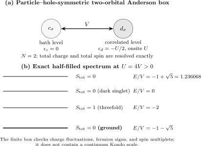
The minimal Anderson box contains one interacting impurity orbital and one bath orbital. At $N=2$ it separates into a threefold triplet and three singlets. The numerical spectrum shown uses $U=4V$; the singlet–triplet splitting approaches $8V^2/U$ for large $U$ but a two-orbital box does not resolve continuum Kondo scaling.

Numerical target at U = 4V

Set

$$V=1, \qquad U=4.$$

The sorted eigenvalues are

$$\begin{array}{c|c|c} \text{energy} & \text{total spin} & \text{degeneracy} \\ \hline -1-\sqrt5 &0&1 \\ -2 &1&3 \\ 0 &0&1 \\ -1+\sqrt5 &0&1 \end{array}$$

or numerically

$$\begin{aligned} E_-/V&=-3.236067977500, \\ E_T/V&=-2.000000000000, \\ E_0/V&=0, \\ E_+/V&=1.236067977500. \end{aligned}$$

The singlet–triplet gap is

$$\frac{\Delta_{ST}}V = \sqrt5-1 = 1.236067977500.$$

For the normalized ground state, particle–hole symmetry gives

$$\langle n_d\rangle =1.$$

The impurity double occupancy is

$$D_d = \frac14 \left( 1-\frac1{\sqrt5} \right) = 0.138196601125.$$

The impurity charge variance is

$$\left\langle (n_d-1)^2 \right\rangle = 2D_d = 0.276393202250.$$

The single-occupation probability, equal here to the local-moment diagnostic, is

$$\begin{aligned} m_{\mathrm{loc}}^2 &= \left\langle n_d-2n_{d\uparrow}n_{d\downarrow} \right\rangle \\ &= \frac12 \left( 1+\frac1{\sqrt5} \right) \\ &= 0.723606797750. \end{aligned}$$

The impurity–bath spin correlation is

$$\begin{aligned} \langle \mathbf S_d\cdot\mathbf S_c \rangle &= -\frac38 \left( 1+\frac1{\sqrt5} \right) \\ &= -0.542705098312. \end{aligned}$$

Define the dimensionless transfer operator

$$T_{dc} = \sum_\sigma \left( d_\sigma^\dagger c_\sigma + c_\sigma^\dagger d_\sigma \right).$$

Then

$$\langle T_{dc}\rangle = -\frac4{\sqrt5} = -1.788854382000.$$

These values were independently checked by constructing the full four-mode Fock-space Hamiltonian and projecting to $N=2$.

Matrix invariants

For the complete six-state block,

$$\operatorname{tr}H_{N=2} = -2U,$$ $$\operatorname{tr}H_{N=2}^2 = U^2+8V^2,$$

and

$$\det H_{N=2} =0.$$

At $U=4V$, these become

$$\operatorname{tr}H_{N=2} = -8V, \qquad \operatorname{tr}H_{N=2}^2 = 24V^2.$$

The zero determinant is physical: the antisymmetric doublon combination is an exact zero-energy singlet in this symmetric two-orbital box.

Benchmark contract

A reproducible implementation should state:

1. mode order, here $(d_\uparrow,d_\downarrow,c_\uparrow,c_\downarrow)$;
2. the fermionic sign convention used to construct creation operators;
3. $V=1$, $U=4$, $\epsilon_d=-2$, and bath energy zero;
4. total particle number $N=2$;
5. whether absolute energies or shifted energies are reported;
6. eigenvalues with the triplet degeneracy resolved;
7. $\langle n_d\rangle$, $D_d$, $m_{\mathrm{loc}}^2$, $\langle\mathbf S_d\cdot\mathbf S_c\rangle$, and $\langle T_{dc}\rangle$;
8. the trace and trace-square invariants.

Agreement on energies but not local observables usually indicates a basis, operator, or eigenvector-normalization error. Agreement on the spectrum after an undocumented energy shift is not enough.

Numerical and Analytical Methods

Numerical renormalization group

NRG maps the bath to a logarithmic Wilson chain and iteratively retains low-energy states. It is especially effective when the target contains exponentially separated impurity scales. Report the discretization parameter, interleaved grids, truncation policy, broadening kernel, and convergence checks.

Continuous-time quantum Monte Carlo

Hybridization- and interaction-expansion algorithms provide finite-temperature imaginary-time observables with statistical error bars. Sign severity depends on model structure. Real-frequency spectra require an additional reconstruction whose prior assumptions and uncertainty should be reported.

Exact diagonalization

ED gives all eigenpairs of a finite bath up to Hilbert-space limits. Its strongest role is transparent symmetry-resolved benchmarking and zero-temperature finite-cluster response. Continuum claims require a bath-fitting and convergence sequence.

Tensor-network impurity solvers

Star-to-chain transformations permit matrix-product-state methods in real or imaginary time. Accuracy is governed by chain length, entanglement growth, bond dimension, time step, and Fourier-window treatment.

Bethe ansatz

Integrable formulations provide exact equilibrium information for specific continuum models. Their assumptions must travel with quoted results, and dynamic quantities may remain difficult even when the spectrum is integrable.

Perturbative and renormalized methods

Weak-$U$, weak-hybridization, large-degeneracy, high-temperature, and low-energy Fermi-liquid expansions each have distinct control parameters. Static Hartree–Fock can display moment-like solutions but is not an exact description of the zero-field finite impurity ground state.

Principal Variants

Infinite-U Anderson model

The doublon is projected out. Empty and singly occupied states still fluctuate, so the local Hilbert space has three states rather than the two states of a fixed spin-$1/2$.

Multiorbital impurity

Crystal fields, Hund exchange, pair hopping, and spin–orbit coupling enlarge the local interaction tensor. Stating only one number $U$ is generally insufficient.

Structured or pseudogapped bath

Energy-dependent $\Gamma(\omega)$ can produce thresholds, bound states, or impurity quantum phase transitions absent from the featureless metallic baseline. The low-energy power law and ultraviolet completion must be specified.

Superconducting bath

Nambu structure and the superconducting gap introduce Andreev and subgap states. Particle number may no longer be the convenient manifest symmetry, although fermion parity remains meaningful.

Nonequilibrium and several leads

Lead labels, chemical potentials, temperatures, switching protocol, and current operator become part of the model. A single equilibrium $\Delta(z)$ is not enough.

Periodic Anderson model

An interacting orbital on every unit cell creates a lattice problem with coherence, band formation, and collective ordering. It is not obtained by solving many independent single impurities unless an explicit approximation such as DMFT supplies that mapping.

Model Boundaries

• Anderson impurity versus Kondo impurity: the Anderson model retains local charge; the Kondo model retains only a fixed spin after controlled projection.
• Anderson impurity versus Hubbard lattice: one interacting site in a bath is not an interacting lattice, even though DMFT relates them self-consistently.
• Anderson impurity versus resonant level: the resonant-level model is the $U=0$ limit, not a generic approximation at strong interaction.
• Anderson impurity versus Anderson localization: they share a name but describe different Hamiltonians and phenomena.
• Coherent bath versus Markovian reservoir: eliminating a bath into a memoryless generator is an additional approximation, not the original closed Hamiltonian.

Common Mistakes

• Specifying $\rho_{\mathrm{bath}}$ but not the hybridization weights $V_k$.
• Treating impurity occupancy as a conserved quantum number.
• Interpreting $\langle n_d\rangle=1$ as proof that charge fluctuations vanish.
• Calling $\Gamma$ a full width when the displayed Green function makes it a half-width.
• Dropping $\Lambda(\omega)$ without stating the wide-band or renormalized-level convention.
• Using the Kondo mapping when either charge gap is comparable to hybridization or temperature.
• Calling finite-bath exact diagonalization the exact continuum solution.
• Assuming Bethe-ansatz integrability supplies every dynamical correlator.
• Reading an unrestricted mean-field moment as exact spontaneous symmetry breaking of one finite impurity.
• Treating the familiar three-feature spectral sketch as universal for every bath and parameter set.
• Calling single-site DMFT exact in arbitrary finite dimension.
• Comparing spectra produced with different energy zeros, broadenings, or sum-rule conventions.

Summary

• The model combines one correlated spinful orbital with a quadratic fermionic bath.
• Total charge is conserved, but impurity charge fluctuates through hybridization.
• The bath is specified locally by $\Delta(z)$ or equivalently by $\Gamma(\omega)$ plus its analytic real part.
• Atomic charge gaps organize empty-orbital, mixed-valence, local-moment, and doubly occupied regimes.
• Particle–hole symmetry fixes average unit occupancy while allowing finite empty and doublon probabilities.
• Atomic, resonant-level, integrable-continuum, finite-bath, and low-energy exact statements have different scopes.
• A Kondo model follows only after both impurity charge excitations are safely eliminated.
• The two-orbital box provides an exact spectrum, spin multiplets, local observables, and large-$U$ exchange check.

Exercises

1. Atomic charge boundaries

For $U\gt0$, compare $E_0$, $E_\sigma$, and $E_2$ and derive the three atomic ground-charge regions. Identify the two degeneracy points.

Solution

The energies are

$$\begin{aligned} E_0&=0, \\ E_\sigma&=\epsilon_d, \\ E_2&=2\epsilon_d+U. \end{aligned}$$

The empty state wins when

$$0\lt\epsilon_d$$

because then $E_0\lt E_\sigma$ and, for repulsive $U$, also $E_0\lt E_2$ in the relevant region. Single occupation wins when

$$\epsilon_d\lt0$$

and

$$\epsilon_d \lt 2\epsilon_d+U,$$

which gives

$$-U\lt\epsilon_d\lt0.$$

Double occupation wins when

$$2\epsilon_d+U \lt \epsilon_d,$$

or

$$\epsilon_d\lt-U.$$

The degeneracy points are $\epsilon_d=0$ and $\epsilon_d=-U$. Hybridization turns these atomic crossings into avoided many-body crossovers for a conventional metallic bath.

2. One-level hybridization function

Take one bath orbital of energy $\epsilon_c$ and hybridization $V$. Compute $\Delta(z)$. Explain why this finite bath does not produce a smooth lifetime width.

Solution

The definition gives

$$\Delta(z) = \frac{\lvert V\rvert^2}{z-\epsilon_c}.$$

Its retarded imaginary part is distributional,

$$\Gamma(\omega) = \pi\lvert V\rvert^2 \delta(\omega-\epsilon_c).$$

The coupled finite system has discrete poles and coherent recurrences. A smooth linewidth emerges only after a continuum limit or an explicitly declared broadening. Adding a plotting kernel changes the visualization, not the exact finite-bath Hamiltonian.

3. Derive the two-orbital singlet block

At particle–hole symmetry and $N=2$, show that the triplets have energy $-U/2$. In the singlet sector, identify the doublon combination that couples to $\lvert S\rangle$ and obtain the $3\times3$ block up to basis phases.

Solution

Every triplet has one particle on the impurity and one on the bath. It therefore contributes impurity energy $-U/2$ and no interaction energy. Spin-conserving hopping cannot connect a total-spin-one state to a same-orbital doublon, which is a singlet. Hence

$$E_T=-\frac U2.$$

The covalent singlet has the same diagonal energy. The two doublons each have zero energy:

$$2\epsilon_d+U=0, \qquad 2\epsilon_c=0.$$

Hybridization connects $\lvert S\rangle$ to one normalized combination of $\lvert D_d\rangle$ and $\lvert D_c\rangle$ with matrix-element magnitude $2V$. The orthogonal combination is dark. After choosing basis phases,

$$H_{S=0} = \begin{pmatrix} -U/2&-2V&0 \\ -2V&0&0 \\ 0&0&0 \end{pmatrix}.$$

The sign of $2V$ changes under a phase reversal of either connected basis state and is not itself an observable.

4. Spectrum and invariants

Factor the $N=2$ characteristic polynomial. Use the spectrum to verify $\operatorname{tr}H$, $\operatorname{tr}H^2$, and $\det H$.

Solution

The triplets contribute the factor

$$\left(E+\frac U2\right)^3.$$

The dark singlet contributes $E$, and the coupled singlet block contributes

$$E^2+\frac U2E-4V^2.$$

Therefore

$$\begin{aligned} P_2(E) ={}& E \left(E+\frac U2\right)^3 \\ &\times \left( E^2+\frac U2E-4V^2 \right). \end{aligned}$$

The eigenvalue sum is

$$\begin{aligned} 3\left(-\frac U2\right) +E_-+E_+ &= -\frac{3U}{2}-\frac U2 \\ &= -2U. \end{aligned}$$

Since

$$\begin{aligned} E_-+E_+ &= -\frac U2, \\ E_-E_+ &= -4V^2, \end{aligned}$$

their squared sum is

$$E_-^2+E_+^2 = \frac{U^2}{4}+8V^2.$$

Adding three triplet squares gives

$$\operatorname{tr}H^2 = U^2+8V^2.$$

The dark zero-energy singlet makes

$$\det H=0.$$

5. Ground-state observables from derivatives

For

$$E_- = -\frac U4 - \sqrt{ \frac{U^2}{16}+4V^2 },$$

use Hellmann–Feynman derivatives along the particle–hole-symmetric line to obtain $D_d$ and $\langle T_{dc}\rangle$. Evaluate them at $U=4V$.

Solution

Along $\epsilon_d=-U/2$,

$$\frac{\partial H}{\partial U} = n_{d\uparrow}n_{d\downarrow} - \frac12n_d.$$

Particle–hole symmetry gives $\langle n_d\rangle=1$, so

$$\frac{\partial E_-}{\partial U} = D_d-\frac12.$$

Differentiating the exact energy yields

$$D_d = \frac14 - \frac{U}{16 \sqrt{U^2/16+4V^2}}.$$

At $U=4V$,

$$D_d = \frac14 \left( 1-\frac1{\sqrt5} \right).$$

Because

$$\frac{\partial H}{\partial V} = T_{dc},$$

another derivative gives

$$\langle T_{dc}\rangle = -\frac{4V}{ \sqrt{U^2/16+4V^2} }.$$

At $U=4V$ this becomes

$$\langle T_{dc}\rangle = -\frac4{\sqrt5}.$$

6. Audit a Kondo reduction

Consider a metallic bath with $U=12\Gamma_0$ and temperature $k_{\mathrm B}T=0.05\Gamma_0$. Compare:

1. $\epsilon_d=-6\Gamma_0$;
2. $\epsilon_d=-0.8\Gamma_0$.

Which point has a parametrically credible spin-only reduction based on the charge-gap test?

Solution

At the symmetric point,

$$\Delta_0 = \Delta_2 = 6\Gamma_0.$$

Both exceed hybridization and temperature by large factors, so a low-energy spin-only reduction is parametrically credible.

At the second point,

$$\Delta_0 = 0.8\Gamma_0, \qquad \Delta_2 = 11.2\Gamma_0.$$

The empty-state gap is comparable to the hybridization scale. Real charge fluctuations are not safely eliminated, even if the average occupancy happens to be near one. This point is closer to mixed valence, and the Anderson charge sectors should be retained.

Cross-Links

• Quantum Dots — confinement, capacitance, addition spectra, and transport-stability diagrams for the device realization.
• Model Encyclopedia Overview — comparison with lattice, gas, pairing, and impurity dossiers.
• Kondo Effect — material realization, transport and spectroscopy diagnostics, screening-cloud evidence, and the heavy-fermion bridge.
• Anderson Impurity Model Preview — atomic thermodynamics, resonant level, spectra, Friedel sum rule, quantum dots, and DMFT.
• Kondo Model — compact spin-only descendant, scaling regimes, and finite Kondo-box benchmark.
• Kondo Model Preview — logarithmic flow, screening, thermodynamics, and local Fermi liquid.
• Effective Hamiltonians in Many-Body Systems — virtual empty and doublon paths in the Kondo reduction.
• Schrieffer–Wolff Transformation — general unitary block diagonalization.
• Green Functions in Many-Body QM — Lehmann representations, sum rules, and addition/removal sectors.
• Spectral Functions — widths, residues, convolution, and spectral diagnostics.
• Fermi-Liquid Theory Preview — low-energy quasiparticle and response language.
• Benchmark Problems — reproducibility contracts for many-body calculations.
• Common Many-Body Hamiltonians — compact formula and convention lookup.

References

1. P. W. Anderson, “Localized Magnetic States in Metals”, Physical Review 124, 41–53 (1961) — original interacting localized-level model and local-moment problem.
2. J. R. Schrieffer and P. A. Wolff, “Relation between the Anderson and Kondo Hamiltonians”, Physical Review 149, 491–492 (1966) — canonical charge-sector elimination and exchange model.
3. D. C. Langreth, “Friedel Sum Rule for Anderson’s Model of Localized Impurity States”, Physical Review 150, 516–518 (1966) — interacting impurity phase-shift relation.
4. F. D. M. Haldane, “Scaling Theory of the Asymmetric Anderson Model”, Physical Review Letters 40, 416–419 (1978) — scale separation and asymmetric-model renormalization.
5. P. B. Wiegmann, “Towards an Exact Solution of the Anderson Model”, Physics Letters A 80, 163–167 (1980) — integrability of a continuum Anderson formulation.
6. A. C. Hewson, The Kondo Problem to Heavy Fermions, Cambridge University Press (1993), doi:10.1017/CBO9780511470752 — standard monograph on Anderson and Kondo impurities, exact limits, and low-energy relations.
7. R. Bulla, T. A. Costi, and T. Pruschke, “Numerical Renormalization Group Method for Quantum Impurity Systems”, Reviews of Modern Physics 80, 395–450 (2008) — Wilson-chain construction, thermodynamics, dynamics, and numerical controls.
8. A. Georges, G. Kotliar, W. Krauth, and M. J. Rozenberg, “Dynamical Mean-Field Theory of Strongly Correlated Fermion Systems and the Limit of Infinite Dimensions”, Reviews of Modern Physics 68, 13–125 (1996) — self-consistent impurity mapping and its exact dimensional limit.
9. Y. Meir and N. S. Wingreen, “Landauer Formula for the Current through an Interacting Electron Region”, Physical Review Letters 68, 2512–2515 (1992) — interacting quantum-dot transport framework.
10. E. Gull, A. J. Millis, A. I. Lichtenstein, A. N. Rubtsov, M. Troyer, and P. Werner, “Continuous-Time Monte Carlo Methods for Quantum Impurity Models”, Reviews of Modern Physics 83, 349–404 (2011) — continuous-time impurity algorithms and error structure.