Photon Number States

A photon number state, or optical Fock state, has a definite number of excitations in one or more specified electromagnetic modes. For one normalized mode $f$,

$$\hat N_f\lvert n_f\rangle = n\lvert n_f\rangle, \qquad n=0,1,2,\ldots .$$

The subscript matters. A photon is an excitation of a mode, and a mode includes its frequency content, spatial profile, polarization, and temporal envelope. The statement “this pulse is a one-photon state” is incomplete until the relevant mode or mode subspace has been identified.

Number states have exact excitation number, vanishing number variance, no first-order field amplitude, and sharply nonclassical counting correlations. Those facts do not imply that:

• a photon is a tiny localized pellet following a trajectory;
• every detector gate returns exactly the prepared photon number;
• a weak laser pulse is a one-photon state;
• a definite-number state possesses an ordinary but unknown optical phase;
• a small measured value of $g^{(2)}(0)$ by itself certifies every desirable property of a single-photon source.

This page develops the optical meaning of Fock states. The oscillator algebra is canonical on Number States, and general many-mode occupation notation is canonical on Fock-Space Number States. The calibrated map from incident occupation statistics to optical detector outcomes belongs on Photon Counting. Measurement records and quantum jumps for a continuously monitored output belong on open-system Photon Counting.

Scope and Operational Questions

The phrase “photon number” can refer to several related but distinct objects:

Question	Mathematical object
How many excitations occupy mode $f$?	eigenvalue of $\hat N_f=\hat a_f^\dagger\hat a_f$
What number would an ideal measurement of that mode return?	distribution $P_f(n)=\langle n_f\vert\rho\vert n_f\rangle$
How many detector events occur in a gate?	a detector-dependent count distribution
How many photons occupy all modes in a set $\mathcal B$?	$\hat N_{\mathcal B}=\sum_{\mu\in\mathcal B}\hat N_\mu$
How many photons leave an open system per unit time?	output flux or counting intensity

Only the first two are intrinsic to the specified field state and mode decomposition. A raw count record also depends on loss, collection, mode-selective filtering, detector efficiency, dark counts, dead time, timing jitter, and number resolution.

The clean model below begins with lossless bosonic modes. Open propagation and detection are introduced as quantum channels and measurements, not silently folded into the definition of the state.

Number States of One Optical Mode

Let $\hat a_f$ annihilate one excitation in a normalized electromagnetic mode $f$, with

$$[\hat a_f,\hat a_f^\dagger]=1.$$

The mode number operator is

$$\hat N_f = \hat a_f^\dagger\hat a_f.$$

Starting from the mode vacuum,

$$\hat a_f\lvert0_f\rangle=0,$$

the normalized number states are

$$\lvert n_f\rangle = \frac{(\hat a_f^\dagger)^n}{\sqrt{n!}} \lvert0_f\rangle.$$

They obey

$$\hat a_f\lvert n_f\rangle = \sqrt n\,\lvert(n-1)_f\rangle,$$ $$\hat a_f^\dagger\lvert n_f\rangle = \sqrt{n+1}\,\lvert(n+1)_f\rangle,$$

and

$$\hat N_f\lvert n_f\rangle = n\lvert n_f\rangle.$$

For an ideal monochromatic normal mode of angular frequency $\omega_f$, the free Hamiltonian contribution is

$$\hat H_f = \hbar\omega_f \left( \hat N_f+\frac12 \right).$$

Thus $\lvert n_f\rangle$ is both a number eigenstate and an energy eigenstate. For a finite-bandwidth traveling wave packet, however, a state with one photon in the packet need not be an exact free-energy eigenstate. Definite excitation number and definite energy are different assertions.

The optical field in a number state

For one mode at a fixed spacetime point, a field quadrature has the form

$$\hat X_\theta = \frac{ \hat a_f e^{-i\theta} + \hat a_f^\dagger e^{i\theta} }{\sqrt2}.$$

Every number state has

$$\langle n_f\vert\hat a_f\vert n_f\rangle=0, \qquad \langle\hat X_\theta\rangle=0.$$

Its quadrature variance is independent of $\theta$:

$$(\Delta X_\theta)^2 = n+\frac12.$$

The mean electric field therefore vanishes, but its fluctuations do not. The state $\lvert n_f\rangle$ is not a classical wave of fixed amplitude whose phase has merely been hidden. Its field statistics differ from those of a phase-randomized classical amplitude.

The vacuum $n=0$ has the minimum oscillator variance. Adding a definite photon number increases both conjugate quadrature variances equally rather than selecting a classical oscillation phase.

One Photon Means One Mode Excitation

A normalized wave-packet mode can be assembled from a continuum of frequency, wavevector, and polarization modes. In schematic notation,

$$\hat a_f^\dagger = \sum_\lambda \int d^3k\, f_\lambda(\mathbf k) \hat a_{\mathbf k\lambda}^\dagger,$$

with

$$\sum_\lambda \int d^3k\, \lvert f_\lambda(\mathbf k)\rvert^2 = 1.$$

The associated one-photon state is

$$\lvert1_f\rangle = \hat a_f^\dagger\lvert0\rangle.$$

Its label $f$ contains the full mode specification. Another normalized mode $g$ has overlap

$$[\hat a_f,\hat a_g^\dagger] = \langle f\vert g\rangle.$$

Consequently,

$$\langle1_f\vert1_g\rangle = \langle f\vert g\rangle.$$

Perfectly distinguishable photons occupy orthogonal modes; perfectly indistinguishable single photons occupy the same mode apart from degrees of freedom deliberately used to label paths or qubits.

A photon does not have to be monochromatic

For free propagation, the wave-packet state evolves as

$$\lvert1_f(t)\rangle = \sum_\lambda \int d^3k\, f_\lambda(\mathbf k) e^{-i\omega_{\mathbf k}t} \hat a_{\mathbf k\lambda}^\dagger \lvert0\rangle.$$

A short pulse requires a bandwidth. Its energy moments are

$$\langle H\rangle = \sum_\lambda \int d^3k\, \hbar\omega_{\mathbf k} \lvert f_\lambda(\mathbf k)\rvert^2,$$

and

$$\begin{aligned} (\Delta H)^2 ={}& \sum_\lambda \int d^3k\, (\hbar\omega_{\mathbf k})^2 \lvert f_\lambda(\mathbf k)\rvert^2 \\ &- \langle H\rangle^2. \end{aligned}$$

The state still has exactly one excitation in the wave-packet subspace while having nonzero energy uncertainty.

Mode basis dependence

Suppose one input mode is transformed into two orthogonal output modes:

$$\hat a_f^\dagger \longmapsto t\,\hat b^\dagger + r\,\hat c^\dagger, \qquad \lvert t\rvert^2+\lvert r\rvert^2=1.$$

Then

$$\lvert1_f\rangle \longmapsto t\lvert1_b,0_c\rangle + r\lvert0_b,1_c\rangle.$$

The total photon number remains exactly one, but neither output port has definite local occupation. This is ordinary unitary mode mixing, not creation or destruction of the photon.

The general basis-dependence of occupation is developed on Mode Occupations.

Many-Mode Optical Fock States

For orthonormal optical modes $f_1,f_2,\ldots$, a multimode number state is

$$\lvert n_1,n_2,\ldots\rangle = \prod_j \frac{ (\hat a_j^\dagger)^{n_j} }{ \sqrt{n_j!} } \lvert0\rangle.$$

It satisfies

$$\hat N_j \lvert n_1,n_2,\ldots\rangle = n_j \lvert n_1,n_2,\ldots\rangle.$$

The total number in the chosen mode set is

$$\hat N_{\mathrm{tot}} = \sum_j\hat N_j.$$

A state may have definite total number without definite occupation of each mode. For example,

$$\lvert\psi\rangle = \frac{ \lvert1_a,0_b\rangle + e^{i\phi}\lvert0_a,1_b\rangle }{\sqrt2}$$

has one photon in total and a meaningful relative phase $\phi$ between paths. This does not contradict the absence of an absolute phase for a single-mode number state. Relative phase resides in coherence between different mode occupations.

Mixed one-photon states

Not every source emitting at most one photon prepares a pure mode $\lvert1_f\rangle$. Conditioned on the one-photon sector, a general state is

$$\rho_1 = \sum_j q_j \lvert1_{f_j}\rangle \langle1_{f_j}\rvert, \qquad \sum_jq_j=1,$$

in its eigenmode decomposition. Its modal purity is

$$\mathcal P_1 = \operatorname{Tr}(\rho_1^2) = \sum_jq_j^2.$$

A source can therefore have nearly perfect photon-number purity and still emit photons in an incoherent mixture of temporal or spectral modes. This distinction is central to two-photon interference.

Photon Number Statistics

For a single selected mode in state $\rho$, the ideal photon-number distribution is

$$P(n) = \langle n\vert\rho\vert n\rangle, \qquad \sum_{n=0}^{\infty}P(n)=1.$$

The moments are

$$\langle \hat N^k\rangle = \sum_{n=0}^{\infty}n^kP(n).$$

For a number state $\lvert n_0\rangle$,

$$P(n)=\delta_{n,n_0},$$

so

$$\langle\hat N\rangle=n_0, \qquad (\Delta N)^2=0.$$

The probability-generating function

$$G(z) = \langle z^{\hat N}\rangle = \sum_{n=0}^{\infty}P(n)z^n$$

is useful because

$$\left. \frac{d^rG}{dz^r} \right|_{z=1} = \langle \hat N(\hat N-1)\cdots(\hat N-r+1) \rangle.$$

These falling-factorial moments are exactly the operator moments naturally selected by ideal absorptive photodetection:

$$\langle\hat N^{\underline r}\rangle = \left\langle (\hat a^\dagger)^r\hat a^r \right\rangle.$$

For $\lvert n_0\rangle$,

$$\langle\hat N^{\underline r}\rangle = \begin{cases} \dfrac{n_0!}{(n_0-r)!}, & r\le n_0, \\[6pt] 0, & r>n_0. \end{cases}$$

There cannot be an $(n_0+1)$-fold ideal absorption coincidence from an $n_0$-photon state.

Variance, Fano factor, and Mandel parameter

Three related statistics are

$$(\Delta N)^2 = \langle\hat N^2\rangle - \langle\hat N\rangle^2,$$ $$F = \frac{(\Delta N)^2}{\langle\hat N\rangle},$$

and

$$Q = \frac{ (\Delta N)^2-\langle\hat N\rangle }{ \langle\hat N\rangle } = F-1.$$

For an exact nonvacuum number state,

$$F=0, \qquad Q=-1.$$

For a Poisson distribution, $F=1$ and $Q=0$. Sub-Poissonian statistics means $F<1$, or equivalently $Q<0$. It is a sufficient signature of nonclassicality for the measured mode under the standard photodetection model.

Normalized intensity correlation

The equal-mode, zero-delay normalized second-order correlation is

$$g^{(2)}(0) = \frac{ \langle \hat a^\dagger\hat a^\dagger\hat a\hat a \rangle }{ \langle\hat a^\dagger\hat a\rangle^2 } = \frac{ \langle\hat N(\hat N-1)\rangle }{ \langle\hat N\rangle^2 }.$$

For $\lvert n\rangle$ with $n\ge1$,

$$g^{(2)}(0) = 1-\frac1n.$$

In particular,

$$g^{(2)}(0)=0$$

for an ideal one-photon state. Two detections from the same single excitation are impossible. For large $n$, $g^{(2)}(0)$ approaches one even though the state remains an exact, highly nonclassical number state. Therefore $g^{(2)}(0)\approx1$ does not by itself prove that light is coherent or classical.

The relation

$$Q = \langle\hat N\rangle \left[ g^{(2)}(0)-1 \right]$$

follows directly from $\hat N^2=\hat N(\hat N-1)+\hat N$. It is valid for a single selected counting mode with finite nonzero mean.

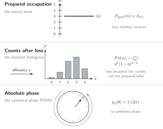
Three complementary statements about an ideal number state. Its prepared occupation is exact, loss converts that delta distribution into a binomial count distribution, and an absolute phase measurement is uniform. A detector histogram is therefore not the same object as the source-state distribution.

Prepared Number Versus Detected Counts

An ideal number measurement projects onto

$$\Pi_n=\lvert n\rangle\langle n\rvert.$$

Real photodetection usually implements a different positive-operator-valued measure after a lossy channel. For a detector with independent efficiency $\eta$ and perfect number resolution, each of the $n$ incident photons is registered with probability $\eta$. The conditional count distribution is

$$\begin{aligned} P(k\mid n) &= \binom nk \eta^k (1-\eta)^{n-k}, \\ &\qquad 0\le k\le n. \end{aligned}$$

For an incident number distribution $P_{\mathrm{in}}(n)$,

$$P_{\mathrm{det}}(k) = \sum_{n=k}^{\infty} \binom nk \eta^k (1-\eta)^{n-k} P_{\mathrm{in}}(n).$$

This is Bernoulli thinning. For an input $\lvert n_0\rangle$,

$$\langle K\rangle = \eta n_0,$$ $$\operatorname{Var}(K) = \eta(1-\eta)n_0.$$

The observed Fano factor and Mandel parameter become

$$F_{\mathrm{det}}=1-\eta, \qquad Q_{\mathrm{det}}=-\eta.$$

Loss weakens sub-Poissonian number squeezing but does not make the detected count distribution a delta function at a smaller integer.

Why normalized correlations can survive loss

Under independent loss,

$$\langle K\rangle = \eta\langle N\rangle,$$

and

$$\langle K(K-1)\rangle = \eta^2 \langle N(N-1)\rangle.$$

Hence

$$g_{\mathrm{det}}^{(2)}(0) = g_{\mathrm{in}}^{(2)}(0)$$

when there are no dark counts, backgrounds, saturation effects, or mode-dependent efficiencies. This useful cancellation does not mean loss is irrelevant: brightness, heralding efficiency, count uncertainty, and higher-order inference all degrade.

On–off detectors

An on–off detector distinguishes no click from at least one click but does not resolve $k=1$ from $k=2$. For an $n$-photon input with no dark counts,

$$P(\text{no click}\mid n) = (1-\eta)^n,$$ $$P(\text{click}\mid n) = 1-(1-\eta)^n.$$

A click therefore does not certify that exactly one photon arrived. Detector tomography, calibrated attenuation, multiplexing, or coincidence measurements may be needed to infer the incident distribution. The number-resolving and threshold POVMs, dark counts, dead time, and detector calibration are developed on optical Photon Counting. Conditional time records and quantum-jump dynamics are treated on open-system Photon Counting.

Number and Optical Phase

A number state has no preferred absolute optical phase. The precise reason is not merely that some heuristic uncertainty product becomes large. The number spectrum is bounded below, and this obstructs an everywhere-defined self-adjoint phase operator satisfying an unrestricted canonical commutator with $\hat N$.

Suppose one naively assumed

$$[\hat N,\hat\Phi]=i\hat I$$

on the number states. Taking the diagonal matrix element in $\lvert n\rangle$ would give

$$\langle n\vert [\hat N,\hat\Phi] \vert n\rangle = 0,$$

whereas the proposed right-hand side gives $i$. The contradiction signals a domain and spectrum problem, not a failure of quantum mechanics.

Phase shifts are well defined

The unitary phase-shift operator is unproblematic:

$$\hat U(\varphi) = e^{-i\varphi\hat N}.$$

It acts on a number state as

$$\hat U(\varphi)\lvert n\rangle = e^{-in\varphi}\lvert n\rangle.$$

This is only a global phase for a single number state, so every measurement probability is invariant under $\varphi$. A superposition of different number states can acquire observable relative phases.

The exponential phase operator is not unitary

A useful number-lowering shift is

$$\hat E = \sum_{n=0}^{\infty} \lvert n\rangle\langle n+1\rvert = (\hat N+1)^{-1/2}\hat a.$$

It obeys

$$\hat E\hat E^\dagger=\hat I,$$

but

$$\hat E^\dagger\hat E = \hat I-\lvert0\rangle\langle0\rvert.$$

The missing inverse at the vacuum boundary prevents $\hat E$ from being a unitary exponential of an ordinary Hermitian phase operator.

Phase POVMs

Optical phase can nevertheless be described operationally by a positive-operator-valued measure. Introduce generalized phase kets

$$\lvert\theta\rangle = \sum_{n=0}^{\infty} e^{in\theta}\lvert n\rangle, \qquad 0\le\theta<2\pi.$$

They are not normalizable Hilbert-space vectors, but they define the canonical phase POVM

$$d\Pi(\theta) = \frac{d\theta}{2\pi} \lvert\theta\rangle\langle\theta\rvert.$$

For a state with number-basis elements $\rho_{mn}=\langle m\vert\rho\vert n\rangle$, the phase probability density is

$$p(\theta) = \frac{1}{2\pi} \sum_{m,n=0}^{\infty} \rho_{mn} e^{i(n-m)\theta}.$$

For $\rho=\lvert n_0\rangle\langle n_0\rvert$,

$$p(\theta)=\frac{1}{2\pi}.$$

Thus every absolute phase is equally likely. More generally, every number-diagonal state has a uniform canonical phase distribution because it contains no coherence between different number sectors.

Pegg–Barnett construction

Pegg and Barnett define phase first in an $(s+1)$-dimensional truncated number space. The orthonormal phase states are

$$\lvert\theta_m^{(s)}\rangle = \frac{1}{\sqrt{s+1}} \sum_{n=0}^{s} e^{in\theta_m} \lvert n\rangle,$$

where

$$\theta_m = \theta_0+\frac{2\pi m}{s+1}, \qquad m=0,\ldots,s.$$

Physical expectation values are calculated at finite $s$, and only then is the limit $s\to\infty$ taken. This produces a consistent Hermitian phase observable within the prescription. It should not be shortened to the claim that an unrestricted canonical $\hat\Phi$ exists on the full oscillator Hilbert space.

What “phase uncertainty” should mean

Phase is periodic, so an ordinary linear variance depends on the branch cut. Useful measures include:

• the canonical phase distribution $p(\theta)$;
• circular moments such as $\langle e^{i\theta}\rangle$;
• the Holevo variance where applicable;
• a specified interferometric phase-estimation error;
• quadrature statistics measured relative to a local oscillator.

For a number state, the first circular moment vanishes and the canonical phase distribution is uniform. Writing

$$\Delta N\,\Delta\Phi\ge\frac12$$

without defining $\Phi$, its domain, and the periodic uncertainty measure is not a reliable statement.

Absolute Phase, Relative Phase, and References

Optical phase is observed relative to a reference mode, path, clock, or local oscillator. Consider

$$\lvert\psi\rangle = \frac{ \lvert1_a,0_b\rangle + e^{i\phi}\lvert0_a,1_b\rangle }{\sqrt2}.$$

The total photon number is exactly one, yet a beam splitter can convert the relative phase $\phi$ into output probabilities. There is no contradiction: $\phi$ relates two amplitudes in a multimode state and is not an absolute single-mode phase.

Likewise, homodyne detection uses a strong local oscillator to define which field quadrature is measured. A phase estimate always inherits assumptions about the reference and mode matching. Removing the reference can turn an apparently phase-coherent description into a number-diagonal reduced state.

Single-Photon Sources

An ideal pulsed single-photon source would produce, on demand, the same pure wave-packet state on every trigger:

$$\rho_{\mathrm{ideal}} = \lvert1_f\rangle\langle1_f\rvert.$$

Real sources are better represented by photon-number sectors,

$$\rho = p_0\rho_0 + p_1\rho_1 + p_2\rho_2 + \cdots,$$

where $\rho_n$ is normalized within the $n$-photon sector and

$$\sum_{n=0}^{\infty}p_n=1.$$

Even this decomposition hides important modal structure: $\rho_1$ may be mixed, and $\rho_2$ may contain photons in distinguishable modes.

Source qualities are multidimensional

A useful source characterization reports several quantities rather than one headline number:

Property	Operational question
preparation probability	how often does a trigger create the desired state?
brightness	how often is a useful photon delivered at a stated reference plane?
multiphoton suppression	how small are $p_{n\ge2}$ or $g^{(2)}(0)$?
collection efficiency	how much emitted light enters the target mode?
heralding efficiency	given a herald, how often is its partner present?
purity	is the one-photon sector a pure spatiotemporal mode?
indistinguishability	do photons from separate trials interfere as identical modes?
repetition rate	how often can a source attempt emission?
stability	do these properties remain constant over the acquisition?

Numbers must be quoted at a stated plane. “Source efficiency” measured at the first lens, fiber output, chip facet, or detector are not interchangeable.

Deterministic emitters

A quantum emitter with at most one excitation can emit at most one photon before it is re-excited. Examples include atoms, ions, molecules, color centers, and semiconductor quantum dots. Under pulsed excitation, the ideal cycle is

$$\lvert g,0\rangle \longrightarrow \lvert e,0\rangle \longrightarrow \lvert g,1_f\rangle.$$

Antibunching follows because the emitter must be excited again before another photon can be emitted. Real imperfections include re-excitation within the same pump pulse, nonradiative decay, dephasing, spectral diffusion, blinking, imperfect collection, and emission into unwanted modes. Photon Antibunching develops the conditional reset dynamics and the measured continuous-wave and pulsed correlation signatures.

A resonator can enhance emission into a selected mode and shape the output wave packet. Cavity-assisted Raman protocols can transfer an atomic excitation into a propagating photon in a controlled temporal mode. These processes connect to Spontaneous Emission and later cavity-QED treatments.

Heralded pair sources

Weak parametric down-conversion or four-wave mixing approximately produces a two-mode squeezed state,

Parametric Down-Conversion owns source geometries, biphoton modes, spectral purity, and heralding metrics. Nonlinear Quantum Optics develops the common susceptibility, phase-matching, and effective-Hamiltonian machinery. The present section keeps the focus on the conditional photon-number state and its imperfections.

$$\begin{aligned} \lvert\Psi\rangle &= \sqrt{1-\lambda^2} \sum_{n=0}^{\infty} \lambda^n \lvert n_s,n_i\rangle, \\ &\qquad 0\le\lambda<1. \end{aligned}$$

Detecting an idler photon heralds the presence of a signal photon. In the weak pump limit, the dominant heralded term is $\lvert1_s\rangle$, but higher pair terms remain:

$$\lvert2_s,2_i\rangle, \quad \lvert3_s,3_i\rangle, \quad\ldots$$

Increasing the pump raises the herald rate and the multipair contamination. Loss and threshold herald detectors make the conditional state more subtle because a single herald click may have originated from several idler photons.

Spectral correlations can also leave the heralded signal in a mixed mode. Engineering the joint spectral amplitude, filtering, or mode-selective detection can improve purity, often at a cost in brightness or heralding efficiency.

Attenuated laser pulses are not single-photon states

A coherent pulse with mean photon number $\mu$ has Poisson statistics,

$$P(n) = e^{-\mu}\frac{\mu^n}{n!}.$$

When $\mu\ll1$,

$$\begin{gathered} P(0)\approx1-\mu, \qquad P(1)\approx\mu, \\ P(2)\approx\frac{\mu^2}{2}. \end{gathered}$$

Most pulses are vacuum, some contain one photon, and a nonzero fraction contain two or more. Attenuation changes $\mu$ but does not convert the coherent state into $\lvert1\rangle$. In particular,

$$g^{(2)}(0)=1$$

for an ideal coherent state at every nonzero amplitude, whereas $g^{(2)}(0)=0$ for $\lvert1\rangle$.

Weak coherent pulses are useful and often experimentally convenient. They should simply be named correctly.

Diagnosing a Single-Photon Source

For a weak source with negligible $p_{n\ge3}$,

$$\langle N\rangle \approx p_1+2p_2,$$

and

$$\langle N(N-1)\rangle \approx 2p_2.$$

Hence

$$g^{(2)}(0) \approx \frac{2p_2}{(p_1+2p_2)^2}.$$

If $p_2\ll p_1$, this is often simplified to

$$g^{(2)}(0) \approx \frac{2p_2}{p_1^2}.$$

The approximation must not be used when multiphoton components are sizable. Moreover, a small $g^{(2)}(0)$ says little about vacuum probability, brightness, spectral purity, or indistinguishability.

Hanbury Brown–Twiss test

Send the source into one input of a balanced beam splitter and place detectors at both outputs. An ideal single-photon input transforms as

$$\lvert1,0\rangle \longmapsto \frac{ \lvert1,0\rangle + i\lvert0,1\rangle }{\sqrt2},$$

for one common phase convention. There is no $\lvert1,1\rangle$ term, so an ideal trial cannot produce a true coincidence between the two outputs.

The ratio of zero-delay coincidences to an appropriate uncorrelated baseline estimates $g^{(2)}(0)$ after corrections and normalization. Background, afterpulsing, detector dead time, timing windows, and source intermittency can bias the estimate. Reporting only a fitted number without the acquisition and normalization model is incomplete.

Hanbury Brown–Twiss Interferometry develops the two-detector geometry, accidental baseline, timing convolution, and continuous-versus-pulsed normalization.

Indistinguishability is a separate test

Two individually antibunched photons may still differ in frequency, temporal shape, polarization, or spatial mode. Hong–Ou–Mandel interference compares two photons and probes their modal overlap. For pure one-photon modes $f$ and $g$, ideal balanced-beam-splitter coincidence probability is

$$P_{\mathrm c} = \frac12 \left( 1-\lvert\langle f\vert g\rangle\rvert^2 \right).$$

Thus perfect mode overlap gives zero coincidences, while orthogonal modes give $1/2$. Source multiphoton terms, loss, detector response, and mixedness alter the observed visibility. Antibunching and indistinguishability answer different questions.

Nonclassicality of Number States

Quantum optics often calls a state classical if it can be written as a statistical mixture of coherent states with a nonnegative regular Glauber–Sudarshan distribution:

$$\rho = \int d^2\alpha\, P(\alpha) \lvert\alpha\rangle\langle\alpha\rvert, \qquad P(\alpha)\ge0.$$

For such a state, normally ordered field moments can be reproduced by a classical random complex amplitude. Number states with $n\ge1$ do not admit such a positive regular representation. Their $P$ distributions are more singular than ordinary probability densities.

Sub-Poissonian fluctuations

For any positive mixture of coherent states, conditional counts are Poissonian and classical intensity fluctuations can only add variance. Consequently,

$$\operatorname{Var}(N) \ge \langle N\rangle$$

under the ideal single-mode photodetection model. An observed

$$\operatorname{Var}(N) < \langle N\rangle$$

therefore rules out that classical model. Exact number states attain the strongest possible suppression, $\operatorname{Var}(N)=0$.

Anticorrelation at a beam splitter

A single classical wave entering a beam splitter produces fields in both outputs. Shot noise from ideal semiclassical photodetection does not create the perfect conditional anticorrelation of an ideal one-photon state. The beam-splitter test made this distinction operational: one excitation is found in one output or the other, never both in the same trial.

For $\lvert n\rangle$, the result

$$g^{(2)}(0)=1-\frac1n<1$$

is likewise incompatible with a positive classical intensity ensemble for that mode.

Wigner-function negativity

In the convention where the vacuum Wigner function is

$$W_0(\alpha) = \frac{2}{\pi} e^{-2\lvert\alpha\rvert^2},$$

the number-state Wigner function is

$$W_n(\alpha) = \frac{2}{\pi} (-1)^n L_n\left(4\lvert\alpha\rvert^2\right) e^{-2\lvert\alpha\rvert^2},$$

where $L_n$ is a Laguerre polynomial. For every $n\ge1$, this function has negative regions. Wigner negativity is another sufficient nonclassicality signature, but it is not equivalent to every other criterion for arbitrary states.

Nonclassical does not mean useful for every task

The label “nonclassical” identifies failure of a specified classical-state model. It does not automatically certify:

• high source brightness;
• low loss;
• pure temporal or spectral mode;
• entanglement;
• metrological advantage under realistic resources;
• compatibility with a particular memory, detector, or network.

Resource claims require an operational task and a complete accounting of state preparation, reference frames, loss, and measurement.

Worked Example: A Lossy Three-Photon State

Send $\lvert3\rangle$ through a channel of transmissivity $\eta$. The output state of the retained mode is number diagonal:

$$\rho_{\mathrm{out}} = \sum_{k=0}^{3} \binom3k \eta^k(1-\eta)^{3-k} \lvert k\rangle\langle k\rvert.$$

The probabilities are

$$P(0)=(1-\eta)^3,$$ $$P(1)=3\eta(1-\eta)^2,$$ $$P(2)=3\eta^2(1-\eta),$$ $$P(3)=\eta^3.$$

The mean and variance are

$$\langle N\rangle=3\eta, \qquad (\Delta N)^2=3\eta(1-\eta).$$

Yet

$$g^{(2)}(0) = \frac{ 3\cdot2\,\eta^2 }{ (3\eta)^2 } = \frac23,$$

independent of $\eta$ in the ideal loss-only model. The output is no longer an exact number state, while its normalized second-order correlation retains the input value.

Worked Example: Heralding with a Threshold Detector

Take the pair state

$$\lvert\Psi\rangle = \sqrt{1-\lambda^2} \sum_{n=0}^{\infty} \lambda^n \lvert n_s,n_i\rangle.$$

An ideal threshold detector on the idler reports “click” for every $n\ge1$. Conditioned on a click, the signal state is

$$\rho_{s\mid\mathrm{click}} = (1-\lambda^2) \sum_{n=1}^{\infty} \lambda^{2(n-1)} \lvert n_s\rangle\langle n_s\rvert.$$

The conditional single-photon weight is

$$P(1\mid\mathrm{click}) = 1-\lambda^2,$$

and the multiphoton weight is

$$P(n\ge2\mid\mathrm{click}) = \lambda^2.$$

Weak pumping suppresses multipair events, but it also lowers the unconditional herald rate. Nonunit idler efficiency further biases the conditional mixture because higher-pair events are more likely to produce at least one detected idler photon.

A Practical Analysis Workflow

When a problem or experiment invokes a photon number state:

1. Define the mode. State the spatial, spectral, temporal, and polarization mode, or define the measured mode subspace.
2. Define the reference plane. Separate generation, collection, propagation, and detector losses.
3. Write the state by number sector. Keep vacuum, one-photon, and multiphoton probabilities explicit.
4. Inspect modal purity. A pure number sector need not be a pure wave-packet mode.
5. Specify the measurement. Distinguish ideal number resolution, on–off clicks, multiplexed detection, and time-resolved counting.
6. Propagate detector effects. Include efficiency, backgrounds, dead time, and timing windows.
7. Choose a diagnostic for the claim. Use $g^{(2)}(0)$ for multiphoton suppression, tomography for the number distribution, and two-photon interference for indistinguishability.
8. State what is not certified. Avoid promoting one statistic into a complete source characterization.

Common Mistakes

Omitting the mode label

The ket $\lvert1\rangle$ is shorthand. Without a mode definition it does not say where, when, at what frequency, or in which polarization the excitation can be coupled or detected.

Confusing source probabilities with count probabilities

Loss converts an incident number state into a mixture at the detector. Detector clicks are outcomes of a measurement model, not direct labels pasted onto the source density operator.

Calling weak coherent light a single photon

A highly attenuated coherent pulse remains a vacuum–one–multiphoton superposition with Poisson statistics. Small mean energy is not definite photon number.

Treating a click as number resolving

An on–off click means one or more absorbed events according to the detector model. It does not distinguish one incident photon from several.

Equating small second-order correlation with high quality

A source can have low $g^{(2)}(0)$ and poor brightness, modal purity, indistinguishability, or stability. State the property actually measured.

Saying a number state has a random classical phase

Uniform phase statistics do not turn a Fock state into a classical phase-randomized wave. The two states have different number and correlation statistics.

Using an unrestricted phase commutator

The lower bound of the number spectrum obstructs a globally canonical self-adjoint phase operator. Use a specified phase POVM, finite-dimensional construction, or interferometric observable.

Confusing total and local occupation

A one-photon superposition across two paths has definite total number but indefinite number in either path. Passive mode mixing preserves total number.

Ignoring multimode mixedness

One photon per trigger does not guarantee that photons from different triggers occupy the same pure temporal and spectral mode.

Interpreting loss invariance too broadly

Ideal $g^{(2)}$ ratios may cancel uniform efficiency, but backgrounds, mode-dependent loss, saturation, and statistical uncertainty do not cancel in general.

Connections

• Photonic Qubits uses these mode and source diagnostics in processor-level encodings, multiplexing, fusion, loss, and throughput budgets.
• Phase-Space Distributions relates number-state parity to Wigner values and compares the corresponding $P$, Wigner, and $Q$ functions.
• Beam Splitters develops number-state splitting, single-photon path amplitudes, and the canonical Hong–Ou–Mandel transformation.
• Quantum Optics supplies the chapter map from field states to transformations and measurements.
• Quantized Electromagnetic Modes derives the oscillator assigned to each radiation mode.
• Number States is the canonical home for one-oscillator ladder algebra.
• Fock-Space Number States develops bosonic and fermionic occupation bases generally.
• Mode Occupations explains why occupation depends on the chosen one-particle basis.
• Coherent Light owns Poisson optical counting, all-order coherence, and realistic laser limits; Coherent States provides the canonical oscillator construction.
• Thermal Light develops geometric occupation statistics, super-Poissonian fluctuations, and intensity bunching.
• Squeezed States: First Encounter contrasts definite number with reduced quadrature noise.
• Entanglement in Quantum Optics treats mode entanglement and optical Bell resources.
• Photon Counting owns continuous count records, detector imperfections, and quantum jumps.

Exercises

1. Number-state field moments

For

$$\hat X = \frac{\hat a+\hat a^\dagger}{\sqrt2},$$

show that in $\lvert n\rangle$,

$$\langle\hat X\rangle=0, \qquad \langle\hat X^2\rangle=n+\frac12.$$

Explain why this does not describe a classical oscillation of unknown phase.

Solution

The ladder operators change number, so orthogonality gives

$$\langle n\vert\hat a\vert n\rangle = \langle n\vert\hat a^\dagger\vert n\rangle = 0.$$

Therefore $\langle\hat X\rangle=0$. Expanding the square,

$$\hat X^2 = \frac12 \left( \hat a^2 + \hat a\hat a^\dagger + \hat a^\dagger\hat a + (\hat a^\dagger)^2 \right).$$

The first and last terms change number by two and have zero diagonal matrix elements. Using

$$\hat a^\dagger\hat a=\hat N, \qquad \hat a\hat a^\dagger=\hat N+1,$$

one obtains

$$\langle\hat X^2\rangle = \frac12 \left( n+1+n \right) = n+\frac12.$$

The state is rotationally symmetric in phase space: every quadrature has the same variance and no quadrature has a nonzero mean. A classical oscillation would require a phase-referenced displacement, represented quantum mechanically by coherence between different number states.

2. Correlations of an exact number state

Derive

$$g^{(2)}(0)=1-\frac1n$$

for $\lvert n\rangle$, and evaluate it for $n=1$, $2$, and $10$.

Solution

Apply the annihilation operators:

$$\hat a\hat a\lvert n\rangle = \sqrt{n(n-1)} \lvert n-2\rangle.$$

Therefore

$$\langle n\vert \hat a^\dagger\hat a^\dagger\hat a\hat a \vert n\rangle = n(n-1).$$

Since $\langle\hat a^\dagger\hat a\rangle=n$,

$$g^{(2)}(0) = \frac{n(n-1)}{n^2} = 1-\frac1n.$$

The requested values are

$$\begin{gathered} g^{(2)}_{n=1}(0)=0, \qquad g^{(2)}_{n=2}(0)=\frac12, \\ g^{(2)}_{n=10}(0)=0.9. \end{gathered}$$

The approach to one at large $n$ does not make the exact number state a coherent state; higher moments and phase-space structure remain different.

3. Loss and number resolution

An ideal $\lvert2\rangle$ state reaches a number-resolving detector with efficiency $\eta=0.6$. Find the probabilities of zero, one, and two counts, the mean count, the variance, and the observed $g^{(2)}(0)$.

Solution

Bernoulli thinning gives

$$P(k\mid2) = \binom2k (0.6)^k(0.4)^{2-k}.$$

Thus

$$\begin{gathered} P(0)=0.16, \qquad P(1)=0.48, \\ P(2)=0.36. \end{gathered}$$

The binomial mean and variance are

$$\langle K\rangle=2(0.6)=1.2,$$ $$\operatorname{Var}(K) = 2(0.6)(0.4) = 0.48.$$

The factorial moment is

$$\langle K(K-1)\rangle = 2P(2) = 0.72.$$

Therefore

$$g^{(2)}(0) = \frac{0.72}{(1.2)^2} = \frac12.$$

It equals the input value, illustrating loss invariance for ideal uniform thinning without background.

4. Uniform phase of a number state

Using the canonical phase POVM, show that every state diagonal in the number basis has a uniform phase distribution.

Solution

Let

$$\rho = \sum_{n=0}^{\infty} p_n\lvert n\rangle\langle n\rvert.$$

Insert $\rho_{mn}=p_n\delta_{mn}$ into

$$p(\theta) = \frac{1}{2\pi} \sum_{m,n} \rho_{mn} e^{i(n-m)\theta}.$$

Only terms with $m=n$ survive:

$$p(\theta) = \frac{1}{2\pi} \sum_n p_n = \frac{1}{2\pi}.$$

The result applies to a pure number state and to any incoherent mixture of number states. A uniform canonical phase distribution therefore does not identify a unique photon-number distribution.

5. One photon at a beam splitter

A photon enters port $a$ of a balanced beam splitter while port $b$ is in vacuum. Use

$$\hat a^\dagger \longmapsto \frac{ \hat c^\dagger+i\hat d^\dagger }{\sqrt2}$$

to find the output state and the photon-number covariance $\operatorname{Cov}(N_c,N_d)$.

Solution

The input is

$$\lvert1_a,0_b\rangle = \hat a^\dagger\lvert0\rangle.$$

After the beam splitter,

$$\lvert\psi_{\mathrm{out}}\rangle = \frac{ \lvert1_c,0_d\rangle + i\lvert0_c,1_d\rangle }{\sqrt2}.$$

Each output has mean occupation

$$\langle N_c\rangle = \langle N_d\rangle = \frac12.$$

There is never one photon in both outputs, so

$$\langle N_cN_d\rangle=0.$$

Hence

$$\begin{aligned} \operatorname{Cov}(N_c,N_d) &= \langle N_cN_d\rangle \\ &\quad- \langle N_c\rangle\langle N_d\rangle \\ &= -\frac14. \end{aligned}$$

The negative covariance expresses output anticorrelation while total number remains exactly one.

6. Weak coherent pulse versus imperfect single-photon source

Compare two pulsed sources with the same mean photon number $\langle N\rangle=0.1$:

1. a coherent state;
2. the mixture $\rho=0.9\lvert0\rangle\langle0\rvert +0.1\lvert1\rangle\langle1\rvert$.

Find $P(2)$ and $g^{(2)}(0)$ for each.

Solution

For the coherent state, $\mu=0.1$ and

$$P_{\mathrm{coh}}(2) = e^{-0.1}\frac{0.1^2}{2} \approx 4.52\times10^{-3}.$$

Every nonvacuum coherent state has

$$g_{\mathrm{coh}}^{(2)}(0)=1.$$

The vacuum–one-photon mixture has

$$P_{\mathrm{mix}}(2)=0.$$

Moreover,

$$\langle N(N-1)\rangle=0,$$

so

$$g_{\mathrm{mix}}^{(2)}(0)=0.$$

Equal mean energy does not imply equal photon statistics. Vacuum probability also does not prevent the conditional nonvacuum output from having perfect multiphoton suppression.

7. Modal purity of a one-photon mixture

A source emits exactly one photon, but its one-photon state is

$$\rho_1 = q\lvert1_f\rangle\langle1_f\rvert + (1-q)\lvert1_g\rangle\langle1_g\rvert,$$

where $\langle f\vert g\rangle=0$. Compute the modal purity and determine its minimum over $q$.

Solution

Orthogonality removes cross terms in $\rho_1^2$:

$$\rho_1^2 = q^2\lvert1_f\rangle\langle1_f\rvert + (1-q)^2 \lvert1_g\rangle\langle1_g\rvert.$$

Therefore

$$\mathcal P_1 = \operatorname{Tr}(\rho_1^2) = q^2+(1-q)^2.$$

Differentiating,

$$\frac{d\mathcal P_1}{dq} = 4q-2,$$

so the minimum occurs at $q=1/2$ and equals

$$\mathcal P_{1,\min} = \frac12.$$

The source has perfect photon-number purity but imperfect modal purity. Photon counting alone cannot distinguish this mixture from a pure one-photon mode.

8. Threshold-heralded pair source

For the ideal pair state on this page, condition on a threshold idler click. Compute the conditional mean signal photon number and $g_s^{(2)}(0)$ in terms of $x=\lambda^2$.

Solution

The conditional distribution is geometric on $n=1,2,\ldots$:

$$P(n\mid\mathrm{click}) = (1-x)x^{n-1}.$$

Its mean is

$$\langle N_s\rangle = \sum_{n=1}^{\infty} n(1-x)x^{n-1} = \frac{1}{1-x}.$$

Using the second derivative of the geometric series,

$$\langle N_s(N_s-1)\rangle = \frac{2x}{(1-x)^2}.$$

Therefore

$$g_s^{(2)}(0) = \frac{ \langle N_s(N_s-1)\rangle }{ \langle N_s\rangle^2 } = 2x = 2\lambda^2.$$

As $\lambda\to0$, the heralded state approaches $\lvert1\rangle$ and $g_s^{(2)}(0)\to0$, while the unconditional probability of obtaining a herald also tends to zero.

References

• R. J. Glauber, “Photon Correlations,” Physical Review Letters 10, 84–86 (1963), doi:10.1103/PhysRevLett.10.84.
• R. J. Glauber, “The Quantum Theory of Optical Coherence,” Physical Review 130, 2529–2539 (1963), doi:10.1103/PhysRev.130.2529.
• L. Mandel and E. Wolf, Optical Coherence and Quantum Optics, Cambridge University Press (1995), doi:10.1017/CBO9781139644105.
• R. Loudon, The Quantum Theory of Light, 3rd ed., Oxford University Press (2000).
• M. O. Scully and M. S. Zubairy, Quantum Optics, Cambridge University Press (1997), doi:10.1017/CBO9780511813993.
• C. C. Gerry and P. L. Knight, Introductory Quantum Optics, Cambridge University Press (2005), doi:10.1017/CBO9780511791239.
• L. Susskind and J. Glogower, “Quantum Mechanical Phase and Time Operator,” Physics 1, 49–61 (1964), doi:10.1063/1.1704154.
• D. T. Pegg and S. M. Barnett, “Unitary Phase Operator in Quantum Mechanics,” Europhysics Letters 6, 483–487 (1988), doi:10.1209/0295-5075/6/6/002.
• D. T. Pegg and S. M. Barnett, “Phase Properties of the Quantized Single-Mode Electromagnetic Field,” Physical Review A 39, 1665–1675 (1989), doi:10.1103/PhysRevA.39.1665.
• L. Mandel, “Sub-Poissonian Photon Statistics in Resonance Fluorescence,” Optics Letters 4, 205–207 (1979), doi:10.1364/OL.4.000205.
• P. Grangier, G. Roger, and A. Aspect, “Experimental Evidence for a Photon Anticorrelation Effect on a Beam Splitter,” Europhysics Letters 1, 173–179 (1986), doi:10.1209/0295-5075/1/4/004.
• M. D. Eisaman, J. Fan, A. Migdall, and S. V. Polyakov, “Invited Review Article: Single-Photon Sources and Detectors,” Review of Scientific Instruments 82, 071101 (2011), doi:10.1063/1.3610677.
• P. Michler, A. Kiraz, C. Becher, W. V. Schoenfeld, P. M. Petroff, L. Zhang, E. Hu, and A. Imamoğlu, “A Quantum Dot Single-Photon Turnstile Device,” Science 290, 2282–2285 (2000), doi:10.1126/science.290.5500.2282.
• A. Kuhn, M. Hennrich, and G. Rempe, “Deterministic Single-Photon Source for Distributed Quantum Networking,” Physical Review Letters 89, 067901 (2002), doi:10.1103/PhysRevLett.89.067901.
• P. Senellart, G. Solomon, and A. White, “High-Performance Semiconductor Quantum-Dot Single-Photon Sources,” Nature Nanotechnology 12, 1026–1039 (2017), doi:10.1038/nnano.2017.218.