Cryogenic and Vacuum Infrastructure

Cryogenic and vacuum infrastructure establishes the physical boundary conditions under which quantum hardware operates. It removes heat and particles, but it also routes control signals, carries vibration, admits radiation, constrains optical access, and determines how quickly a system can be serviced. A refrigerator or vacuum chamber is therefore not a passive container around the processor. It is part of the processor’s open-system environment.

The central discipline of this page is to distinguish nominal infrastructure specifications from conditions at the quantum degree of freedom:

• refrigerator base temperature is not automatically qubit temperature;
• a chamber’s gauge pressure is not automatically the local collision environment at the trap;
• installed cooling power is not available cooling power after wiring and active dissipation;
• a high pump speed is not the effective speed through a narrow conductance;
• a long single-particle lifetime does not guarantee high whole-array survival;
• low vibration at the floor does not guarantee low relative motion between an optical phase reference and the device.

Last reviewed: 10 August 2026. Published cooling limits, atom-array lifetimes, radiation-mitigation results, and cryogenic-control demonstrations are date-sensitive. Vendor stage labels and nameplate powers are useful design inputs, not portable performance claims.

Purpose and Canonical Scope

This page owns the systems-level infrastructure contract for quantum information hardware:

• staged refrigeration and stage-wise heat accounting;
• thermal occupation and effective device temperature;
• conductive, radiative, optical, and dissipative heat paths;
• cryogenic wiring, attenuation, amplification, and thermalization;
• vibration, electromagnetic, magnetic, infrared, and ionizing-radiation control;
• quantum-hardware consequences of vacuum gas loads, conductance, pumping, residual species, and collisions;
• diagnostics, uncertainty, cooldown or pumpdown time, regeneration, uptime, and serviceability;
• comparison of infrastructure burdens across hardware platforms.

Vacuum Technology owns the general introduction to pressure, mean free path, pressure classes, pumps, gauges, chamber practice, and historical experiments. This page uses those ideas only where they enter a quantum-system resource or error ledger. Control, Readout, and Calibration owns waveform delivery, detector inference, transfer-function calibration, feedback, and drift management. Individual platform pages own device physics. The planned materials and fabrication page owns defects, surfaces, processing, and package materials as fabrication questions.

This is an infrastructure overview, not a construction, operating, or safety manual. Cryogens, compressed gases, high voltage, strong magnets, ionizing radiation, lasers, vacuum vessels, pumps, and oxygen-displacement hazards require institution-specific engineering controls and trained personnel.

The Infrastructure Contract

A useful infrastructure description begins at the laboratory boundary and ends at a declared quantum degree of freedom. It should identify:

1. every thermal stage and its measured temperature under operation;
2. available cooling power and the passive and active load at each stage;
3. every electrical, optical, mechanical, and fluid connection crossing a stage;
4. the noise temperature, attenuation, gain, filtering, and isolation of each signal path;
5. device-package thermalization and the thermometer locations;
6. magnetic, electric, infrared, ionizing-radiation, acoustic, and vibration environments;
7. chamber gas loads, conductances, pumps, gauges, and residual-gas species;
8. local collision, loss, reaction, and contamination observables;
9. cooldown, pumpdown, bakeout, regeneration, calibration, and recovery time;
10. uncertainty, drift, acceptance criteria, and operating duty cycle.

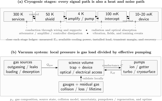
Infrastructure must be closed as a resource ledger. In a cryostat, every control path is also a heat and noise path through finite-capacity stages. In a vacuum system, the science volume is set by local gas loads and conductance-limited pumping, not by pump nameplate speed alone. Device thermometry, vibration spectra, residual-gas analysis, and quantum-object lifetime measurements test the boundary conditions that matter.

A compact performance vector is

$$\begin{aligned} \mathbf I = \big(&T_i,\dot Q_{i,\mathrm{avail}},\dot Q_{i,\mathrm{load}}, \bar n_{\mathrm{mode}},S_T,S_B,S_x,\\ &p_j,S_{\mathrm{eff}},Q_{\mathrm{gas}}, \Gamma_{\mathrm{coll}},\tau_{\mathrm{loss}}, t_{\mathrm{cycle}},A_{\mathrm{up}}\big), \end{aligned}$$

where the index $i$ labels thermal stages, $j$ labels residual-gas species, $S_T$, $S_B$, and $S_x$ denote temperature, magnetic-field, and displacement noise spectra, $t_{\mathrm{cycle}}$ is an infrastructure service cycle such as cooldown plus validation, and $A_{\mathrm{up}}$ is operational availability. The vector is intentionally not reduced to one score.

Why Quantum Hardware Is Environment-Sensitive

The same environmental variable can enter several error mechanisms. A higher temperature can increase equilibrium excitation, quasiparticle density, Johnson noise, blackbody transitions, desorption, and mechanical drift. Residual gas can eject a neutral atom, reorder an ion crystal, react with an ion, contaminate a surface, or scatter a beam. Vibration can modulate an optical phase, a trap position, a cavity length, a magnetic field, or a microwave connection.

The relevant comparison is always between an environmental rate or energy scale and the operation:

$$\begin{aligned} k_BT &\quad \text{versus} \quad \hbar\omega,\\ \Gamma_{\mathrm{coll}}^{-1} &\quad \text{versus} \quad t_{\mathrm{run}},\\ S_x(\omega) &\quad \text{versus the control sensitivity},\\ \dot Q_{\mathrm{load}} &\quad \text{versus} \quad \dot Q_{\mathrm{avail}}. \end{aligned}$$

An infrastructure requirement is therefore task-specific. A dilution refrigerator designed for a slowly swept transport device, a fast superconducting processor, and a microwave–optical converter may share a base temperature while requiring very different wiring, filtering, optical access, heat lift, and stability.

Cryogenic Boundary Conditions

Temperature suppresses thermal occupation

For a bosonic mode of angular frequency $\omega$ in equilibrium at temperature $T$,

$$\bar n_{\mathrm{th}} = \frac{1} {\exp\!\left(\hbar\omega/k_BT\right)-1}.$$

At microwave frequencies, kelvin-scale radiation contains many photons. A $5\,\mathrm{GHz}$ mode has $\hbar\omega/k_B\approx0.240\,\mathrm K$: its equilibrium occupation is about $16$ at $4\,\mathrm K$, about $0.10$ at $100\,\mathrm{mK}$, and about $6\times10^{-6}$ at $20\,\mathrm{mK}$. The exponential improvement is why millikelvin operation matters for superconducting and many semiconductor qubits.

The equation is not a thermometer calibration. A mode coupled weakly to a cold package but strongly to a warmer control line can have an effective occupation far above the value inferred from the mixing-chamber thermometer. Conversely, active reset can prepare a qubit colder than a simple equilibrium model would suggest. Population thermometry, sideband asymmetry, resonator dephasing, or another device-relevant observable is needed to infer the actual state.

Thermal and Vacuum Noise develops the canonical quantum-noise distinction. Thermal Density Operators owns the equilibrium state.

Cooling power is a function, not a label

A modern dry dilution refrigerator commonly uses a pulse-tube cooler to provide tens-of-kelvin and few-kelvin stages, then a circulating $^3\mathrm{He}$–$^4\mathrm{He}$ mixture to reach millikelvin temperatures. Typical named stages include:

Approximate stage	Representative infrastructure role
$300\,\mathrm K$	room-temperature control, pumps, compressors, laser and data systems
$30$–$80\,\mathrm K$	first radiation shield, initial cable interception
$3$–$5\,\mathrm K$	second shield, cryogenic amplifiers, circulators, cryopumps, superconducting magnets
$0.5$–$1\,\mathrm K$	still or intermediate heat interception
$50$–$200\,\mathrm{mK}$	cold plate, further line thermalization and filtering
$5$–$30\,\mathrm{mK}$	mixing chamber, quantum processor, cold attenuators and filters

These are representative functions, not universal temperature bands. The installed options, helium circulation, magnetic field, orientation, cabling, optical load, and upstream stage temperatures change the load curve.

At sufficiently low temperature, an idealized dilution-unit cooling power can be written

$$\dot Q_{\mathrm{mix}} = \dot n_3 \left( 94T_{\mathrm{mix}}^2 - 12T_{\mathrm{in}}^2 \right),$$

with temperatures in kelvin, molar $^3\mathrm{He}$ flow $\dot n_3$ in $\mathrm{mol\,s^{-1}}$, and the numerical coefficients in $\mathrm{J\,mol^{-1}\,K^{-2}}$. If the incoming concentrated phase is well precooled so that $T_{\mathrm{in}}\approx T_{\mathrm{mix}}$, the familiar low-temperature estimate is

$$\dot Q_{\mathrm{mix}} \approx 82\,\dot n_3 T_{\mathrm{mix}}^2.$$

Real performance also depends on heat exchangers, boundary resistance, circulation stability, parasitic heat leaks, and the thermal resistance between the mixing chamber and device. A quoted base temperature is usually measured near zero added load. Scaling must use the full load curve and an engineering margin.

Stage-wise heat balance

For thermal stage $i$, steady operation requires

$$\begin{aligned} \dot Q_{i,\mathrm{load}} &= \dot Q_{i,\mathrm{cond}} +\dot Q_{i,\mathrm{rad}} \\ &\quad +\dot Q_{i,\mathrm{diss}} +\dot Q_{i,\mathrm{opt}} \\ &\quad +\dot Q_{i,\mathrm{other}} < \dot Q_{i,\mathrm{avail}}. \end{aligned}$$

The margin should remain positive during simultaneous operation, not only at idle. Fast pulse sequences, readout amplifiers, heaters, switches, magnetic coils, optical beams, mechanical motion, and regeneration cycles can create bursty or slowly varying loads. A stage can satisfy its average budget while exceeding a transient temperature or recovery-time requirement.

Heat Paths

Conduction through supports and wiring

For a uniform link of length $L$ and cross-sectional area $A$ connecting temperatures $T_c$ and $T_h$,

$$\dot Q_{\mathrm{cond}} = \frac{A}{L} \int_{T_c}^{T_h} k(T)\,dT,$$

where $k(T)$ is the material’s thermal conductivity. At cryogenic temperatures, room-temperature material tables can be badly misleading: purity, alloying, work hardening, superconducting transitions, plating, and geometry matter.

Low-conductivity alloys reduce passive heat leaks but can add electrical loss. High-conductivity copper provides strong thermal anchoring but also transports heat efficiently if it bypasses an intermediate stage. Superconducting conductors suppress electrical resistance below their transition but do not eliminate phonon heat conduction, connector losses, or heat carried by other materials in a cable.

Thermal interception turns one large temperature span into several smaller spans. Each cable, braid, support, waveguide, fibre, capillary, and shaft should have a declared thermal path and anchor. Counting only coaxial lines while ignoring shields, dielectrics, connectors, DC looms, and mechanical supports does not close the ledger.

Radiation

For two surfaces represented by an effective emissivity $\epsilon_{\mathrm{eff}}$ and area $A$, a useful first estimate is

$$\dot Q_{\mathrm{rad}} = \epsilon_{\mathrm{eff}}\sigma A \left(T_h^4-T_c^4\right).$$

Radiation shields intercept room-temperature power at stages with much larger cooling capacity before it reaches millikelvin components. Geometry, view factors, apertures, surface finish, multilayer insulation, seams, cable ports, and optical windows determine the actual load. A direct line of sight can defeat an otherwise excellent shield.

The same principle applies spectrally. Microwave filtering does not guarantee infrared shielding. Infrared photons can break Cooper pairs in superconductors, while room-temperature blackbody radiation can drive atomic or molecular transitions. A credible system specifies the relevant spectral band and path.

Active dissipation

Control power is intentionally dissipated in attenuators, resistive wiring, filters, switches, terminations, amplifiers, heaters, and electronics. For an electrical element,

$$P_{\mathrm{Joule}} = I_{\mathrm{rms}}^2R = \frac{V_{\mathrm{rms}}^2}{R}.$$

This elementary equation becomes a systems problem because the dissipation must be assigned to a thermal stage and duty cycle. A pulse attenuated by $20\,\mathrm{dB}$ deposits most of its incident power as heat at that attenuator. Moving attenuation colder improves the noise temperature seen by the device but consumes scarcer cold-stage cooling power.

Optical absorption deserves the same accounting. A fibre may conduct little heat yet deliver microwatts or milliwatts of optical power to a millikelvin absorber. Scattered trapping light can heat a vacuum enclosure or charge a dielectric. Optical readout, photonic links, and transducers must report absorbed power and recovery as well as delivered photons.

Signal Lines Are Thermal Reservoirs

Attenuation thermalizes only when the attenuator is thermalized

An ideal passive attenuator with power transmission $\eta$ at physical temperature $T_a$ transforms a mode occupation approximately as

$$\bar n_{\mathrm{out}} = \eta\bar n_{\mathrm{in}} + (1-\eta)\bar n_{\mathrm{th}}(T_a).$$

Cascading stages gives

$$\begin{aligned} \bar n_N &= \eta_{1:N}\bar n_0 \\ &\quad+ \sum_{i=1}^{N} (1-\eta_i)\bar n_{\mathrm{th}}(T_i) \eta_{i+1:N}, \\ \eta_{a:b} &\equiv \prod_{j=a}^{b}\eta_j, \qquad \eta_{N+1:N}\equiv1. \end{aligned}$$

Attenuation near the device suppresses upstream noise most effectively, but it also dissipates control power at the coldest stage. Distributed attenuation is therefore a compromise among thermal occupation, pulse amplitude, bandwidth, cooling power, and component reliability.

A metal attenuator bolted to a plate is not automatically at the plate’s effective noise temperature. Contact resistance, connector heating, dielectric loss, insufficient dwell time, and poorly thermalized internal resistive films can matter. In situ noise or qubit thermometry tests the complete chain.

Different lines require different contracts

Line type	Primary function	Infrastructure tension
microwave drive	coherent fast control	low thermal noise versus cold attenuation and pulse power
flux or gate-bias line	DC and low-frequency control	filtering versus rise time; conductor heat leak versus resistance
readout output	carry weak signals outward	reverse noise, gain, isolation, amplifier dissipation
trap RF and electrode lines	confinement and shuttling	high voltage or current, filtering, dissipation, vibration and pickup
optical fibre or free-space beam	control, readout, networking	optical absorption, blackbody path, charging, alignment and vibration
thermometer and heater wiring	measure and stabilize temperature	self-heating, calibration, thermal lag and added wiring

Input and output chains are asymmetric. Readout often needs a near-quantum- limited parametric amplifier, isolators or circulators, and a higher-power amplifier at a warmer stage. Each component has finite reverse isolation, insertion loss, saturation power, bandwidth, magnetic sensitivity, and heat load. Interconnects and Transduction owns the end-to-end quantum-link channel; this page owns how the cryogenic environment constrains that link.

Multiplexing and cryogenic electronics move costs

Frequency, time, code, or switch multiplexing can reduce the number of lines crossing the cryostat. Cryogenic CMOS, superconducting digital logic, local microwave sources, and optical links can move control functions closer to the device. None removes cost; they exchange:

• passive cable conduction for local active power;
• room-temperature bandwidth for cryogenic switching and calibration;
• line count for crosstalk, insertion loss, and failure modes;
• latency for serialization or local processing;
• accessible serviceable electronics for less accessible cold electronics.

The right question is not “How many wires per qubit?” in isolation. It is whether the complete stage-wise power, bandwidth, noise, latency, area, and reliability budget closes for the intended error-correction cycle.

Shielding and Environmental Stability

Electromagnetic and infrared shielding

A practical enclosure usually combines conductive shields, absorptive infrared treatment, filtered feedthroughs, light-tight seams, and carefully defined grounds. The details depend on frequency:

• low-frequency electric fields enter through bias lines, ground loops, and moving charges;
• radio-frequency interference couples through apertures, cable shields, and common impedance;
• microwave photons propagate through intended and parasitic modes;
• infrared radiation enters through seams, connectors, fibres, windows, and warm surfaces.

Shielding is a transfer function, not a material name. It should be validated in the installed configuration across the relevant band. Adding lossy material without thermalizing it can replace one radiation source with another.

Magnetic environment

Magnetic shielding, field coils, trapped flux, magnetized hardware, current return paths, and moving ferromagnetic objects can all affect qubits. The required quantity may be static field, gradient, drift, or spectral density. Superconducting shields can expel or trap flux depending on cooldown history; high-permeability shields can saturate and are temperature dependent.

Hybrid systems expose a sharp integration problem: spin ensembles, ions, or topological-material proposals may require finite magnetic field while nearby superconducting circuits require extremely low field. Spatial separation, compensation coils, nested shields, field-compatible materials, and cooldown protocols become part of the architecture.

Vibration and acoustics

Closed-cycle cryocoolers contain periodic pressure oscillations and machinery that can transmit vibration. Pumps, compressors, building motion, cooling water, acoustic noise, and cable forces add further paths. The relevant observable is often relative displacement:

$$\delta\phi(t) = \mathbf k_{\mathrm{eff}}\!\cdot\! \delta\mathbf x(t)$$

for an optical phase, or a sensitivity-weighted displacement spectrum for a trap, cavity, or package. Isolation stages, flexible thermal links, remote motors, exchange-gas interfaces, rigid common-mode optical mounting, and active stabilization can reduce coupling. A single root-mean-square number can hide narrow spectral lines that coincide with control or trap frequencies, so spectra and measurement bandwidth are preferable.

Ionizing radiation and correlated errors

Environmental gamma rays, radioactive impurities, cosmic-ray secondaries, and stress-release events can deposit energy in a superconducting substrate. The resulting high-energy phonons and nonequilibrium quasiparticles can produce errors correlated across millimetres and milliseconds. This is qualitatively different from a small increase in independent $T_1$ error.

Experiments have linked ionizing events to correlated charge jumps, quasiparticle bursts, and relaxation errors. Mitigations under study include radiopure materials, shielding, phonon sinks, gap engineering, substrate segmentation, event detection, and decoder awareness. No single shielding number establishes fault-tolerant adequacy: terrestrial gamma backgrounds and penetrating cosmic components respond differently, and mitigation must be tested at the logical-cycle level.

Vacuum as a Quantum-Hardware Resource

Pressure is shorthand for a gas distribution

For a dilute ideal gas species $j$ at temperature $T_j$,

$$n_j = \frac{p_j}{k_BT_j}.$$

The total pressure $p=\sum_jp_j$ does not determine collision physics without composition. Hydrogen, helium, water, hydrocarbons, source atoms, and reactive species have different masses, cross sections, sticking probabilities, chemical effects, and gauge sensitivities. A hot atomic source can also create a strongly non-equilibrium directional flux for which a single gas temperature is inadequate.

The generic pressure and mean-free-path foundations live in Vacuum Technology. For trapped quantum hardware, the more direct observable is often the collision rate.

Collision-limited loss and interruption

For a trapped particle interacting with background species $j$,

$$\Gamma_{\mathrm{coll}} = \sum_j n_j \left\langle \sigma_j(v_{\mathrm{rel}})v_{\mathrm{rel}} \right\rangle.$$

If every relevant collision causes loss and other loss processes are absent,

$$P_{\mathrm{surv}}(t) = e^{-\Gamma_{\mathrm{coll}}t}, \qquad \tau_{\mathrm{vac}} = \Gamma_{\mathrm{coll}}^{-1}.$$

Real systems require more structure. A shallow neutral-atom tweezer may lose an atom after nearly any energetic background collision. A deep ion trap may retain the ion but suffer a crystal reordering, a chemical reaction, motional heating, or a temporary interruption. Glancing collisions may remain below a loss threshold. The measured lifetime is therefore a trap- and species-dependent pressure proxy, not a universal conversion.

For $N$ independent trapped particles with identical lifetime $\tau$, the probability that no particle is lost during interval $t$ is

$$P_0(t) = \exp\!\left(-\frac{Nt}{\tau}\right).$$

This scaling explains why a lifetime that looks generous for one atom can be an architectural bottleneck for a large array. Correlated gas bursts, loading-source operation, spatial pressure gradients, and continuous replacement invalidate the simplest independent model and must be reported separately.

Gas Loads and Effective Pumping

The throughput balance

In a well-mixed volume with total gas throughput $Q_{\mathrm{gas}}$ and effective pumping speed $S_{\mathrm{eff}}$, the steady-pressure estimate is

$$p \approx \frac{Q_{\mathrm{gas}}}{S_{\mathrm{eff}}}.$$

The gas load may be decomposed as

$$\begin{aligned} Q_{\mathrm{gas}} &= Q_{\mathrm{out}} +Q_{\mathrm{leak}} +Q_{\mathrm{perm}} \\ &\quad +Q_{\mathrm{source}} +Q_{\mathrm{desorb}} -Q_{\mathrm{getter}}. \end{aligned}$$

where outgassing, real or virtual leaks, permeation, atomic sources, light- or particle-induced desorption, and distributed getter pumping can all matter. Signs and units must be consistent; vacuum throughput is often quoted in $\mathrm{Pa\,m^3\,s^{-1}}$ or $\mathrm{mbar\,L\,s^{-1}}$.

For a surface of area $A$ with specific outgassing rate $q$,

$$Q_{\mathrm{out}} = qA.$$

Outgassing depends on material, surface treatment, cleaning, bake history, time, temperature, absorbed water, hydrogen diffusion, polymers, lubricants, wiring, adhesives, and trapped volumes. A chamber-wall specification alone does not characterize the assembled apparatus.

Conductance limits the pump seen by the experiment

If a pump of speed $S_p$ connects to the science volume through a molecular- flow conductance $C$, then

$$\frac{1}{S_{\mathrm{eff}}} = \frac{1}{S_p} + \frac{1}{C}.$$

A pump with $S_p\gg C$ is conductance limited: $S_{\mathrm{eff}}\approx C$. Narrow tubes, elbows, valves, shields, baffles, windows, and differential-pumping apertures can therefore dominate. The local pressure near the trap can differ from the gauge pressure, especially near a source or through a low-conductance path.

Vacuum design commonly combines pumps with different roles:

• turbomolecular pumps establish high vacuum during pumpdown;
• ion pumps provide clean continuous pumping for many UHV systems;
• non-evaporable getters pump many active gases without moving parts but have species-dependent performance and finite capacity;
• titanium sublimation pumps create fresh reactive surfaces;
• cryosurfaces pump by condensation or adsorption when species and temperature permit;
• differential pumping separates a high-flux loading region from a cleaner science region.

This list is orientation, not a pump-selection guide. Vacuum Technology remains the canonical general page.

Cryopumping is powerful and selective

Cold surfaces can suppress warm-wall outgassing and provide large distributed pumping speed. Whether a gas is condensed, adsorbed, or reflected depends on surface temperature, material, coverage, and species. Hydrogen and especially helium remain difficult at temperatures where water and many heavier gases are efficiently trapped. Sorbents and getters can extend performance.

Cryopumps have finite capacity. Warming a saturated surface can release stored gas, so regeneration and warm-up must be controlled and instrumented. Temporary power loss or an unplanned warm surface can change the residual-gas composition long before a room-temperature gauge reports a simple steady state.

Chamber Interfaces and Optical Access

A quantum vacuum chamber is a network of compromises:

• large numerical aperture improves imaging and photon collection;
• short working distance improves optical resolution;
• windows and glass cells add permeation, charging, birefringence, coatings, thermal stress, and restricted bake temperature;
• nearby electrodes improve trapping and control but increase surface-field sensitivity;
• atom sources improve reload rate but add heat and gas load;
• many feedthroughs improve control but add leaks, outgassing, heat paths, and service complexity;
• smaller volume can pump down quickly but may constrain shields, optics, and replaceable modules.

Optical access must be specified geometrically and spectrally: clear aperture, numerical aperture, working distance, wavelength range, polarization properties, wavefront error, coating behavior, viewport temperature, and line-of-sight blackbody or contamination paths. “Full optical access” is not a single transferable metric.

Loading should be included in the operating cycle. Ovens, dispensers, ablation, photoionization, and magneto-optical traps can raise pressure or deposit material. A platform that reaches excellent base pressure only when its source is off may still be useful, but reload time and recovery must enter the availability model.

Vacuum Diagnostics

Gauges are species- and location-dependent

Ionization gauges, extractor gauges, residual-gas analyzers, spinning-rotor gauges, capacitance gauges, and cold-atom standards operate in different regimes. Their readings can depend on gas species, calibration, geometry, temperature, X-ray limits, electron-stimulated desorption, pumping by the gauge, and conductance to the science volume.

A responsible report states:

• gauge type, location, gas calibration, and operating state;
• whether the value is total or partial pressure;
• whether the loading source, lasers, RF, and cryocooler were operating;
• whether thermal-transpiration or temperature corrections matter;
• the uncertainty or at least the dominant systematic limits.

A residual-gas analyzer helps identify species but is itself a hot-filament and electron-impact device that can perturb a delicate vacuum. It is often most useful during commissioning and fault diagnosis rather than continuous operation next to the quantum system.

The quantum object can be the local sensor

Trap loss, ion-crystal collision events, chemical products, clock shifts, and heating can probe the local environment. Cold-atom vacuum standards make this principle metrological by using calculated and measured collision-rate coefficients. For a known species mixture,

$$p = \frac{k_BT\,\Gamma_{\mathrm{loss}}} {\left\langle\sigma v\right\rangle}$$

in the simplest single-species, unit-loss-probability model.

This inference requires a declared trap depth, collision model, other loss channels, gas temperature, and uncertainty. Agreement between a remote gauge and a trapped-particle lifetime is evidence that a vacuum model is plausible; disagreement is often valuable localization information.

Coupled Cryogenic–Vacuum Systems

Cryogenic and vacuum design cannot be optimized independently.

Vacuum enables thermal isolation

The insulating vacuum around a cryostat suppresses gas conduction and convection. Residual gas can still matter during initial cooldown, a leak, or intentional exchange-gas operation. Radiation shields and low-conductivity supports then set much of the remaining passive load.

Cold surfaces reshape the vacuum

Cooling changes sticking coefficients, vapor pressures, desorption rates, and gas distribution. A cold science region can have much lower local pressure than a warm gauge region. It can also accumulate a hidden gas inventory. Pressure inferred during operation and gas released during warm-up answer different questions.

Mechanical isolation competes with thermal conductance

A thick high-purity copper link conducts heat well but can transmit force and vibration. A flexible braid reduces mechanical coupling but adds thermal resistance and possible microphonic motion. Exchange gas can carry heat across a mechanically soft gap at some temperatures, but its pressure and composition must be controlled. Every vibration-isolation element belongs in the thermal model, and every thermal link belongs in the vibration model.

Optical access competes with shielding

A large warm window provides a radiation view factor. Cold baffles, spectral filters, shutters, nested windows, and carefully placed objectives can intercept radiation, but they add absorption, aberration, drift, and serviceability costs. Cryogenic neutral-atom experiments make this tradeoff especially visible: long lifetime and reduced blackbody radiation are useful only if imaging, trapping, Rydberg control, and field compensation remain adequate.

Platform Infrastructure Profiles

Platform	Characteristic boundary condition	Major infrastructure burdens	Device-relevant observables
superconducting circuits	millikelvin modes with very low microwave and quasiparticle occupation	dilution refrigeration, dense RF/DC wiring, attenuation, isolation, magnetic and infrared shielding, radiation mitigation	qubit excited-state population, resonator thermal occupation, stage loads, quasiparticle and correlated-event rates
silicon spin qubits	sub-kelvin electron reservoirs and stable electrostatic potentials	dilution refrigeration, dense DC/RF wiring, filtering, cryogenic electronics, magnetic field and low charge noise	electron temperature, tunnel broadening, charge stability, gate-line noise, magnet drift
microwave bosonic modes	low occupation and high internal quality factor	millikelvin cavity thermalization, low-loss seams, pump filtering, ancilla reset, readout isolation	mode occupation, lifetime, dephasing, pump-induced heating, ancilla population
trapped ions	UHV or XHV with stable fields and optical phase	vacuum chamber, pumps or cryopumping, RF/DC feedthroughs, optical access, atom source, vibration and magnetic control	collision and reordering rates, chemical reactions, motional heating, optical-path motion, ion lifetime
neutral atoms and molecules	low collision loss with large optical access	UHV or cryogenic vacuum, high-power traps, loading sources, windows or in-vacuum optics, field control	single-particle lifetime, whole-array survival, imaging survival, pressure recovery, blackbody transition rate
defect and solid-state spins	platform-dependent temperature and optical environment	cryostats for many high-coherence or telecom experiments, microwave and optical access, magnetic stability	spin temperature, spectral diffusion, optical linewidth, collection stability
photonic processors and detectors	often ambient optical processing but cryogenic single-photon detection	fibre routing, detector cryocoolers, blackbody filtering, vibration and timing stability	system detection efficiency, dark counts, dead time, temperature and count-rate dependence
topological-material proposals	low temperature, magnetic field, clean interfaces, charge stability	dilution refrigeration, filters, magnets, shielding, extensive DC/RF access	hard-gap stability, parity lifetime, poisoning rate, local electron temperature

The table does not rank platforms. It shows why “operates at room temperature” or “needs a refrigerator” is too coarse for architecture comparison. A photonic processor may avoid millikelvin logic while relying on cryogenic detectors. An atomic processor may avoid dilution refrigeration while requiring extensive lasers, vacuum, stabilization, and optical power. A cryogenic ion or neutral-atom system can trade added refrigeration and vibration work for lower collision rates and blackbody fields.

Performance and Reporting Vector

Cryogenic quantities

A reproducible cryogenic report should include:

• loaded temperature of every relevant stage and thermometer location;
• cooling-power curves or measured margin at the operating point;
• passive and active heat-load estimates by component class;
• wiring materials, counts, thermal anchors, attenuation, filtering, and insertion loss;
• device or mode thermometry rather than plate temperature alone;
• cooldown time, equilibrium time, temperature excursions, and recovery;
• vibration spectra, magnetic drift, and environmental correlations;
• operating duty cycle and rejected or unstable intervals.

Vacuum quantities

A reproducible vacuum report should include:

• chamber geometry relevant to conductance and local sources;
• pumps, estimated or measured effective speeds, and operating states;
• materials, seals, cleaning, bake, activation, and regeneration history;
• total pressure, partial pressures, gauge type, calibration gas, and location;
• source-on and source-off pressure or lifetime behavior;
• collision, loss, reaction, or reordering rates measured at the quantum object;
• pumpdown, reload, recovery, maintenance, and availability.

Uncertainty and drift

Thermometers have calibration uncertainty, magnetic-field dependence, self-heating, and thermal lag. Vacuum gauges have species sensitivity, location bias, calibration uncertainty, and lower-pressure limits. Lifetime fits depend on censoring, correlated loss, loading fluctuations, and competing processes. Error bars should follow the inferred quantity through the model.

Peak performance from a selected cooldown is different from sustained performance across cooldowns. Infrastructure is mature when it is measurable, repeatable, diagnosable, and serviceable, not merely when one record is obtained.

Evidence Through August 2026

The examples below establish different pieces of the infrastructure contract. They should not be combined into a fictional single system.

Cryogenic wiring has demonstrated finite architecture-specific limits

A 2019 superconducting-circuit infrastructure study operated a wired setup for 50 qubits at $14\,\mathrm{mK}$, measured passive and active line loads, and projected support for at least 150 qubits while explicitly setting aside space constraints. It established a disciplined stage-wise method, not a universal refrigerator capacity.

A 2025 study measured the thermal conductivity and electrical resistance of a specific high-density coaxial cable and modeled a particular large dilution refrigerator. It estimated a roughly 200-qubit theoretical limit from cooling power and a practical limit around 140 after margin and cold-stage component space. Those numbers are conclusions about the stated wiring and architecture, not a platform ceiling. Multiplexing, different cables, cryogenic electronics, photonic control links, or different refrigerator staging change the result and introduce other costs.

Thermal photons remain an in situ problem

Cryogenic attenuator and resonator experiments have shown that residual microwave photons can limit superconducting-qubit dephasing and that improved thermalization can increase coherence. Recent theory and measurements continue to emphasize an inherent tension: a control line must transmit a deliberate drive while suppressing broadband thermal noise. Nominal attenuation and plate temperature are insufficient without a calibrated line model and a device-level check.

Radiation creates nonlocal fault mechanisms

Experiments from 2020 onward linked ionizing radiation to elevated quasiparticle density, correlated charge jumps, and relaxation bursts in superconducting devices. Large-array measurements resolved chip-scale events lasting milliseconds. Studies through 2025 directly correlated subsets of events with cosmic-ray detectors and separated some cosmogenic and terrestrial contributions. These results establish radiation as a relevant correlated error channel; they do not establish one universally sufficient shield or decoder response.

Cryogenic ion systems combine XHV, wiring, and vibration control

A 2019 cryogenic trapped-ion apparatus routinely held more than 100 $^{171}\mathrm{Yb}^+$ ions for hours and inferred extremely low background pressure through elastic and inelastic collision observations. A 2021 closed-cycle surface-trap apparatus supported 100 low-frequency lines and eight RF or microwave lines, retained more than $1.3\,\mathrm W$ of cooling power at $5\,\mathrm K$, and reported residual vibration on the order of $10\,\mathrm{nm}$ root mean square. These are complete apparatus results at their demonstrated scales, not evidence that vacuum, optical access, and wiring remain constant under arbitrary QCCD expansion.

Room-temperature and cryogenic atom arrays make different trades

A 2025 room-temperature apparatus trapped more than 6,100 caesium atoms and reported a vacuum-limited single-atom lifetime of $22.9(1)\,\mathrm{min}$, along with qubit coherence, imaging, and transport metrics. The work also emphasized that no-loss probability becomes increasingly demanding with array size.

Cryogenic optical-tweezer experiments reported single-atom lifetimes up to $6000\,\mathrm s$ in 2021 and $3000\,\mathrm s$ in a 2025 high-optical-access Rydberg platform with a $4\,\mathrm K$ cryopumping surface and a colder-than- $50\,\mathrm K$ enclosure. A July 2026 preprint reported up to two-hour vacuum-limited lifetimes for $^{88}\mathrm{Sr}$ while retaining external optical access. The last result is promising but remains a preprint as of this review. Lifetime alone does not establish gate fidelity, array size, blackbody-transition suppression, reload strategy, or sustained availability.

Evidence Ladder

Infrastructure evidence should progress through:

1. component property: conductivity, emissivity, outgassing, pump speed, attenuation, gain, or vibration transmissibility;
2. installed subsystem: measured stage load, local pressure, shield transfer function, or line noise;
3. device-relevant boundary: qubit temperature, mode occupation, collision rate, field spectrum, or optical-path stability;
4. simultaneous operation: all control, readout, loading, and cooling functions active together;
5. scale and duration: representative line count, particle number, cycle rate, and run length;
6. repeatability: multiple cooldowns, bakes, chambers, modules, or service interventions;
7. logical or task effect: measured impact on accepted cycles, logical error, throughput, or time to solution.

A component record at step 1 cannot be promoted directly to a processor claim at step 7.

Design and Validation Workflow

1. Declare the quantum object and task. Specify frequency, trap depth, operation time, accepted temperature, pressure, field, and vibration sensitivities.
2. Draw every boundary crossing. Include wires, shields, dielectrics, fibres, supports, windows, fluids, pumps, sources, and service ports.
3. Build stage-wise thermal and gas-flow models. Keep component identities and units visible.
4. Assign passive, active, transient, and fault loads. Include simultaneous worst credible operation, not only idle averages.
5. Place sensors where the model can fail. Stage thermometers and remote gauges are necessary but rarely sufficient.
6. Commission one subsystem at a time. Measure blank refrigerator loads, cable trees, chamber outgassing, pump conductance, vibration, and shields before adding device complexity.
7. Validate at the quantum object. Use excitation, dephasing, loss, collision, reordering, or spectroscopy observables.
8. Stress the operating envelope. Sweep duty cycle, line power, source state, pump state, optical power, array size, and environmental disturbances.
9. Measure recovery and drift. Record cooldown, pumpdown, warm-up, regeneration, reload, recalibration, and fault-recovery times.
10. Publish the acceptance rule. State which temperature, pressure, lifetime, margin, uncertainty, and availability qualify a run.

Common Mistakes

Equating base temperature with device temperature

The coldest thermometer can be well anchored while a qubit, electron reservoir, cable mode, or package remains warmer. Use a device-relevant thermometer and report the operating load.

Quoting cooling power without temperature

Cooling power is strongly temperature dependent. “One milliwatt of cooling” is meaningless without stage, temperature, load curve, and installed options.

Counting lines but not heat and bandwidth

Two wiring schemes with the same line count can differ greatly in conductor materials, attenuation, pulse dissipation, readout hardware, multiplexing, crosstalk, and serviceability.

Treating attenuation as free refrigeration

An attenuator both replaces upstream noise with its own thermal noise and dissipates signal power. Its stage, physical thermalization, frequency response, and duty cycle matter.

Treating total pressure as collision risk

Collision rates depend on partial pressures, relative velocities, cross sections, trap depth, and the event definition. Gauge location and source state can dominate the inference.

Using pump nameplate speed at the science volume

Finite conductance can make the effective speed much smaller. Report the geometry or measured response connecting the pump to the quantum object.

Calling long single-particle lifetime scalable

Whole-array survival decreases with particle number and run time. Reload, replacement, loss detection, erasure handling, and recovery determine the architecture-level cost.

Ignoring warm-up and regeneration

Cryosurfaces store gas, absorbers store heat, and materials change after thermal cycling. Recovery from a fault or service event is part of availability.

Reporting vibration without the relevant transfer

Floor motion, cold-head motion, package motion, and optical-reference motion are different observables. Report spectra at the points and frequencies that couple to the operation.

Combining best values from incompatible apparatuses

A record atom lifetime, line density, cooling power, optical aperture, and vibration floor may come from different systems and mutually conflicting design choices. Compare complete installed contracts.

Exercises

1. Thermal occupation of a microwave mode

A $5.0\,\mathrm{GHz}$ resonator is alternately coupled to baths at $4.0\,\mathrm K$, $100\,\mathrm{mK}$, and $20\,\mathrm{mK}$. Estimate the equilibrium mean photon occupation at each temperature. Use $h\nu/k_B\approx0.240\,\mathrm K$.

Solution

Use

$$\bar n = \frac{1}{e^{0.240/T}-1}.$$

The three values are approximately

$$\begin{array}{c|c} T & \bar n\\ \hline 4.0\,\mathrm K & 16.2\\ 0.100\,\mathrm K & 0.100\\ 0.020\,\mathrm K & 6.2\times10^{-6} \end{array}$$

Cooling from $4\,\mathrm K$ to $100\,\mathrm{mK}$ changes the mode from many-photon thermal occupation to a small but non-negligible occupation. Reaching $20\,\mathrm{mK}$ suppresses equilibrium occupation by another four orders of magnitude. A measured excess would indicate a warmer effective reservoir or non-equilibrium excitation.

2. Conductive heat leak

A support between $4.0\,\mathrm K$ and $0.10\,\mathrm K$ has $A/L=1.0\times10^{-6}\,\mathrm m$ and $k(T)=aT$ with $a=2.0\times10^{-2}\,\mathrm{W\,m^{-1}\,K^{-2}}$. Estimate the conducted heat.

Solution

Integrate the temperature-dependent conductivity:

$$\begin{aligned} \dot Q &= \frac{A}{L} \int_{0.10}^{4.0}aT\,dT\\ &= \frac{A}{L}\frac{a}{2} \left(4.0^2-0.10^2\right). \end{aligned}$$

Numerically,

$$\dot Q \approx 1.60\times10^{-7}\,\mathrm W = 0.160\,\mu\mathrm W.$$

That can be small at a kelvin stage and significant at a millikelvin stage. The calculation also shows why the actual low-temperature conductivity and geometry are needed.

3. Cascaded cryogenic attenuation

A $5\,\mathrm{GHz}$ input mode begins at $300\,\mathrm K$, for which $\bar n_0\approx1250$. It passes through three ideal $20\,\mathrm{dB}$ attenuators at $4\,\mathrm K$, $100\,\mathrm{mK}$, and $20\,\mathrm{mK}$. Each has $\eta=0.01$. Use the occupations from Exercise 1 and estimate the final occupation.

Solution

Apply

$$\bar n_{\mathrm{out}} = 0.01\bar n_{\mathrm{in}} +0.99\bar n_{\mathrm{th}}$$

at each stage. After the $4\,\mathrm K$ attenuator,

$$\bar n_1 \approx 0.01(1250)+0.99(16.2) \approx 28.5.$$

After the $100\,\mathrm{mK}$ attenuator,

$$\bar n_2 \approx 0.01(28.5)+0.99(0.100) \approx 0.384.$$

After the $20\,\mathrm{mK}$ attenuator,

$$\begin{aligned} \bar n_3 &\approx 0.01(0.384)+0.99(6.2\times10^{-6}) \\ &\approx 3.85\times10^{-3}. \end{aligned}$$

Sixty decibels of total attenuation is not enough information by itself; its distribution among temperatures controls the result. Real components add frequency dependence and imperfect thermalization.

4. Radiation-shield staging

Take $\epsilon_{\mathrm{eff}}=0.05$ and $A=0.050\,\mathrm{m^2}$. Estimate the radiative load on a $4\,\mathrm K$ surface if it sees $300\,\mathrm K$ directly. Then estimate the load if a $50\,\mathrm K$ shield blocks that view. Use $\sigma=5.67\times10^{-8}\,\mathrm{W\,m^{-2}\,K^{-4}}$.

Solution

The direct estimate is

$$\begin{aligned} \dot Q_{300\to4} &\approx 0.05(0.050)\sigma \left(300^4-4^4\right) \\ &\approx 1.15\,\mathrm W. \end{aligned}$$

With a $50\,\mathrm K$ shield, the $4\,\mathrm K$ stage sees

$$\begin{aligned} \dot Q_{50\to4} &\approx 0.05(0.050)\sigma \left(50^4-4^4\right) \\ &\approx 0.89\,\mathrm{mW}. \end{aligned}$$

The shield moves most of the load to a warmer stage with greater cooling capacity. Real multilayer geometries require view factors, apertures, and temperature-dependent emissivity.

5. Collision-limited lifetime

Suppose one residual species has pressure $p=1.0\times10^{-10}\,\mathrm{Pa}$ at $300\,\mathrm K$, effective cross section $\sigma=1.0\times10^{-18}\,\mathrm{m^2}$, and mean relative speed $500\,\mathrm{m\,s^{-1}}$. Assume every collision causes loss. Estimate the number density, collision rate, and lifetime.

Solution

The density is

$$\begin{aligned} n &= \frac{p}{k_BT} \\ &\approx \frac{10^{-10}} {(1.38\times10^{-23})(300)} \\ &\approx 2.4\times10^{10}\,\mathrm{m^{-3}}. \end{aligned}$$

Then

$$\Gamma = n\sigma v \approx 1.2\times10^{-5}\,\mathrm{s^{-1}},$$

so

$$\tau = \Gamma^{-1} \approx 8.3\times10^4\,\mathrm s \approx 23\,\mathrm h.$$

The result is model dependent: real cross sections depend on species and speed, and not every collision necessarily has the same observable outcome.

6. Conductance-limited pumping

A pump has nameplate speed $S_p=100\,\mathrm{L\,s^{-1}}$ but connects to the science chamber through a path of molecular-flow conductance $C=10\,\mathrm{L\,s^{-1}}$. Find the effective pumping speed.

Solution

Use

$$\frac{1}{S_{\mathrm{eff}}} = \frac{1}{100} + \frac{1}{10}.$$

Thus

$$S_{\mathrm{eff}} \approx 9.09\,\mathrm{L\,s^{-1}}.$$

The effective speed is close to the conductance, not the pump nameplate speed. Replacing the pump by a much larger one would produce little improvement unless the connecting conductance also changed.

7. Outgassing-limited pressure

A chamber has internal area $A=2000\,\mathrm{cm^2}$ and specific outgassing rate $q=1.0\times10^{-10}\,\mathrm{mbar\,L\,s^{-1}\,cm^{-2}}$. If $S_{\mathrm{eff}}=100\,\mathrm{L\,s^{-1}}$ and all other gas loads are ignored, estimate the steady pressure.

Solution

The gas throughput is

$$Q_{\mathrm{out}} = qA = 2.0\times10^{-7}\,\mathrm{mbar\,L\,s^{-1}}.$$

Therefore

$$p \approx \frac{Q_{\mathrm{out}}}{S_{\mathrm{eff}}} = 2.0\times10^{-9}\,\mathrm{mbar}.$$

The calculation is only a steady-state estimate. Time-dependent water desorption, hydrogen diffusion, source operation, and species-dependent pump speed can change both pressure and composition.

8. Whole-array survival

An array contains $N=6000$ atoms, each with independent vacuum lifetime $\tau=1200\,\mathrm s$. What is the probability that no atom is lost during a $1.0\,\mathrm s$ interval?

Solution

The no-loss probability is

$$P_0 = \exp\!\left(-\frac{Nt}{\tau}\right) = e^{-5} \approx 6.7\times10^{-3}.$$

Although a 20-minute single-atom lifetime sounds long, a 6000-atom array is very unlikely to remain completely full for one second under the independent model. Useful architectures therefore need longer lifetime, shorter loss-sensitive intervals, replacement, erasure handling, or a task that does not require zero loss everywhere.

9. Stage margin

A $20\,\mathrm{mK}$ stage has $20\,\mu\mathrm W$ available cooling power. Static package and support loads use $7\,\mu\mathrm W$; 120 lines contribute $50\,\mathrm{nW}$ each; cold readout components dissipate $1.5\,\mu\mathrm W$; and control pulses add an average $2.0\,\mu\mathrm W$. Find the remaining margin and its fraction of available power.

Solution

The line load is

$$120(50\,\mathrm{nW}) = 6.0\,\mu\mathrm W.$$

The total load is

$$\dot Q_{\mathrm{load}} = 7+6+1.5+2 = 16.5\,\mu\mathrm W.$$

The margin is

$$20-16.5 = 3.5\,\mu\mathrm W,$$

or $17.5\%$ of the available power. Whether that is adequate depends on load uncertainty, transients, degradation, and the permitted temperature rise.

10. Audit an infrastructure claim

A report states: “The processor is at $10\,\mathrm{mK}$ and operates in $10^{-12}\,\mathrm{mbar}$ vacuum, so thermal and collision errors are negligible.” List at least six missing checks.

Solution

A defensible audit asks at least:

1. Where are the thermometer and vacuum gauge located?
2. Were the values measured with all control, readout, loading, and optical systems operating?
3. What are the qubit, electron, or mode effective temperature and excited population?
4. What gas species dominate, and how is the gauge calibrated for them?
5. What are the local collision, loss, reaction, or reordering rates?
6. What are the cooling-power and effective-pumping margins?
7. What drift, vibration, radiation, and transient events occur?
8. What uncertainty and acceptance criteria apply?
9. Are the results repeatable across cooldowns or bakes?
10. What fraction of scheduled time satisfies the conditions?

The quoted numbers are useful boundary measurements, but they do not alone bound every thermal or collision error seen by the quantum system.

References

1. F. Pobell, Matter and Methods at Low Temperatures, 3rd ed. (Springer, 2007), doi:10.1007/978-3-540-46360-3.
2. C. Enss and S. Hunklinger, Low-Temperature Physics (Springer, 2005), doi:10.1007/b137878.
3. G. K. White and P. J. Meeson, Experimental Techniques in Low-Temperature Physics, 4th ed. (Oxford University Press, 2002).
4. K. Uhlig, “$^3$He/$^4$He dilution refrigerator with pulse-tube refrigerator precooling,” Cryogenics 42, 73–77 (2002), doi:10.1016/S0011-2275(02)00002-4.
5. S. Krinner et al., “Engineering Cryogenic Setups for 100-Qubit Scale Superconducting Circuit Systems,” EPJ Quantum Technology 6, 2 (2019), doi:10.1140/epjqt/s40507-019-0072-0.
6. N. Raicu et al., “Cryogenic Thermal Modeling of Microwave High Density Signaling,” EPJ Quantum Technology 12, 124 (2025), doi:10.1140/epjqt/s40507-025-00427-1.
7. J.-H. Yeh et al., “Microwave Attenuators for Use with Quantum Devices below 100 mK,” Journal of Applied Physics 121, 224501 (2017), doi:10.1063/1.4984894.
8. Z. Wang et al., “Cavity Attenuators for Superconducting Qubits,” Physical Review Applied 11, 014031 (2019), doi:10.1103/PhysRevApplied.11.014031.
9. S. Simbierowicz et al., “Inherent Thermal-Noise Problem in Addressing Qubits,” PRX Quantum 5, 030302 (2024), doi:10.1103/PRXQuantum.5.030302.
10. R. Barends et al., “Minimizing Quasiparticle Generation from Stray Infrared Light in Superconducting Quantum Circuits,” Applied Physics Letters 99, 113507 (2011), doi:10.1063/1.3638063.
11. A. P. Vepsäläinen et al., “Impact of Ionizing Radiation on Superconducting Qubit Coherence,” Nature 584, 551–556 (2020), doi:10.1038/s41586-020-2619-8.
12. C. D. Wilen et al., “Correlated Charge Noise and Relaxation Errors in Superconducting Qubits,” Nature 594, 369–373 (2021), doi:10.1038/s41586-021-03557-5.
13. M. McEwen et al., “Resolving Catastrophic Error Bursts from Cosmic Rays in Large Arrays of Superconducting Qubits,” Nature Physics 18, 107–111 (2022), doi:10.1038/s41567-021-01432-8.
14. X. Li et al., “Cosmic-Ray-Induced Correlated Errors in a Superconducting Qubit Array,” Nature Communications 16, 4677 (2025), doi:10.1038/s41467-025-59778-z.
15. K. Jousten, ed., Handbook of Vacuum Technology, 2nd ed. (Wiley-VCH, 2016), doi:10.1002/9783527688265.
16. J. F. O’Hanlon, A User’s Guide to Vacuum Technology, 3rd ed. (Wiley, 2003), doi:10.1002/0471467162.
17. J. M. Lafferty, ed., Foundations of Vacuum Science and Technology (Wiley, 1998).
18. J. A. Fedchak et al., “Outgassing Rate Comparison of Seven Geometrically Similar Vacuum Chambers of Different Materials and Heat Treatments,” Journal of Vacuum Science and Technology B 39, 024201 (2021), doi:10.1116/6.0000657.
19. D. S. Barker et al., “Precise Quantum Measurement of Vacuum with Cold Atoms,” Review of Scientific Instruments 93, 121101 (2022), doi:10.1063/5.0120500.
20. D. S. Barker et al., “Accurate Measurement of the Loss Rate of Cold Atoms Due to Background Gas Collisions for the Quantum-Based Cold Atom Vacuum Standard,” AVS Quantum Science 5, 035001 (2023), doi:10.1116/5.0147686.
21. G. Pagano et al., “Cryogenic Trapped-Ion System for Large Scale Quantum Simulation,” Quantum Science and Technology 4, 014004 (2019), doi:10.1088/2058-9565/aae0fe.
22. M. F. Brandl et al., “Cryogenic Setup for Trapped Ion Quantum Computing,” Review of Scientific Instruments 87, 113103 (2016), doi:10.1063/1.4966970.
23. T. Dubielzig et al., “Ultra-Low-Vibration Closed-Cycle Cryogenic Surface-Electrode Ion Trap Apparatus,” Review of Scientific Instruments 92, 043201 (2021), doi:10.1063/5.0024423.
24. P. Micke et al., “Closed-Cycle, Low-Vibration 4 K Cryostat for Ion Traps and Other Applications,” Review of Scientific Instruments 90, 065104 (2019), doi:10.1063/1.5088593.
25. C. Monroe et al., “Large-Scale Modular Quantum-Computer Architecture with Atomic Memory and Photonic Interconnects,” Physical Review A 89, 022317 (2014), doi:10.1103/PhysRevA.89.022317.
26. H. J. Manetsch et al., “A Tweezer Array with 6,100 Highly Coherent Atomic Qubits,” Nature 647, 60–67 (2025), doi:10.1038/s41586-025-09641-4.
27. K.-N. Schymik et al., “Single Atoms with 6000-Second Trapping Lifetimes in Optical-Tweezer Arrays at Cryogenic Temperatures,” Physical Review Applied 16, 034013 (2021), doi:10.1103/PhysRevApplied.16.034013.
28. Z. Zhang et al., “High Optical Access Cryogenic System for Rydberg Atom Arrays with a 3000-Second Trap Lifetime,” PRX Quantum 6, 020337 (2025), doi:10.1103/PRXQuantum.6.020337.
29. A. Kumar et al., “A Cryogenic Neutral-Atom Platform with Full Optical Access and 2-Hour Trap Lifetime,” arXiv:2607.12988 (2026), doi:10.48550/arXiv.2607.12988.
30. A. Potočnik et al., “Millikelvin Temperature Cryo-CMOS Multiplexer for Scalable Quantum Device Characterisation,” Quantum Science and Technology 7, 015004 (2022), doi:10.1088/2058-9565/ac29a1.
31. F. Lecocq et al., “Control and Readout of a Superconducting Qubit Using a Photonic Link,” Nature 591, 575–579 (2021), doi:10.1038/s41586-021-03268-x.
32. L. Vogl et al., “Experimental Setup for the Combined Study of Spin Ensembles and Superconducting Quantum Circuits,” Cryogenics 153, 104378 (2026), doi:10.1016/j.cryogenics.2026.104378.

Further Connections

• Hardware Overview places infrastructure inside the complete encoding–control–readout architecture.
• Metrics for Quantum Hardware connects boundary conditions to component, channel, logical, throughput, and workload metrics.
• Control, Readout, and Calibration owns transfer functions, detector inference, calibration dependencies, drift monitoring, and feedback.
• Vacuum Technology owns the general pressure, mean-free-path, pump, gauge, and chamber foundations.
• Superconducting Qubits develops millikelvin microwave processors, packaging, readout chains, correlated errors, and surface-code relevance.
• Silicon Spin Qubits develops electron-temperature, dense-gate, magnet, charge-noise, and cryogenic-controller constraints.
• Trapped-Ion Qubits owns ion encodings, motional gates, shuttling, collision consequences, and QCCD architecture.
• Neutral-Atom and Rydberg Qubits owns loading, rearrangement, optical control, Rydberg gates, located loss, and zone-based processing.
• Photonic Qubits develops optical sources, circuits, loss, feed-forward, and cryogenic detector requirements.
• Interconnects and Transduction develops accepted-input-to-usable-output links, carrier conversion, added noise, heat, and duty cycle.