Neutral-Atom and Rydberg Qubits

Purpose and Canonical Scope

Neutral-atom processors store quantum information in internal states of atoms held by optical tweezers. The atoms can remain weakly interacting while they store information, be moved into a useful geometry, and be coupled strongly for a short time through highly excited Rydberg states. The same ingredients support two rather different operating modes: gate-based quantum processing and programmable analog many-body dynamics.

This page is the canonical architecture-level guide. It owns the connections among:

• atomic storage, auxiliary, interaction, and readout states;
• stochastic loading, fluorescence imaging, rearrangement, and replenishment;
• one-qubit control and native Rydberg-mediated entangling operations;
• geometric reachability, parallel gate scheduling, and coherent transport;
• digital circuits, analog simulation, and the boundary between them;
• loss, leakage, erasure conversion, mid-circuit readout, and reset;
• zone-based architectures, control infrastructure, throughput, and quantum error correction.

It does not duplicate the underlying AMO physics. Optical Tweezers owns tight-focus trapping, quantized motion, loading, imaging, cooling, rearrangement, and coherent transport. Rydberg Atoms owns state selection, excitation, field compensation, lifetime, detection, and pair-potential calibration. Rydberg Blockade owns the two-atom blockade Hamiltonian, collective bright states, finite-blockade corrections, and constrained many-body dynamics. The open-system platform page owns master-equation models for imaging, trap scattering, dephasing, Rydberg decay, and atom loss. Here those ingredients are assembled into a processor contract.

The field is moving quickly. Record array sizes, gate fidelities, logical qubit counts, and error-correction demonstrations are therefore dated evidence, not permanent properties of the platform. Any comparison should use Metrics for Quantum Hardware and state the species, array, protocol, active subset, uncertainty, postselection rule, and date.

The Architecture Contract

A neutral atom is reproducible because its internal spectrum is fixed by its species and isotope. A neutral-atom computer is not specified by that fact alone. It must implement a complete map

$$\begin{gathered} \text{logical instruction} \\ \downarrow \\ \text{atom assignment and geometry} \\ \text{with a zone schedule} \\ \downarrow \\ \text{trap, microwave, and Raman waveforms} \\ \text{plus Rydberg waveforms} \\ \downarrow \\ \text{internal and motional dynamics} \\ \text{with interaction dynamics} \\ \downarrow \\ \text{image or detector record} \\ \text{and classical decision} \end{gathered}$$

A complete platform description identifies at least these layers:

Layer	Required specification
atom	species, isotope, level structure, branching ratios, wavelengths, polarizabilities
encoding	computational states, auxiliary states, leakage manifold, phase convention
confinement	static and moving traps, depth, frequencies, temperature, differential light shifts
loading	source, site occupation, image classifier, rearrangement graph, reservoir policy
control	microwave or Raman rotations, local addressing, Rydberg excitation, pulse synchronization
interaction	selected Rydberg levels, pair potentials, blockade graph, gate or analog Hamiltonian
movement	pick-up, transport, handoff, drop-off, trajectory conflicts, coherence and loss
observation	basis mapping, fluorescence method, loss discrimination, crosstalk, latency
graph	pair reachability, simultaneous gate sets, movement cost, disabled sites and zones
infrastructure	vacuum, lasers, modulators, objectives, cameras, fields, timing, thermal control
operations	calibration graph, scheduler, decoder, drift policy, data provenance, rollback

Several counts that appear similar must remain separate:

1. Trap sites are optical potential minima, whether occupied or not.
2. Loaded atoms are particles detected in those sites.
3. Encoded qubits have been prepared in a declared computational subspace.
4. Calibrated qubits meet stated control and readout criteria.
5. Active qubits participate in the reported operation or circuit.
6. Simultaneously entangled qubits participate in one concurrent gate layer or analog evolution.
7. Logical qubits are encoded objects with a specified code and decoder.

An array containing thousands of coherent atomic qubits can establish storage, imaging, transport, and global-control scale without demonstrating thousands of simultaneous high-fidelity entangling gates. Conversely, a smaller active zone can perform sophisticated logical circuits while a larger reservoir and storage array remain idle. Both are meaningful achievements; they answer different architectural questions.

Atomic Encodings and Functional States

Storage and motion

For $N$ trapped atoms, a useful uncoupled model is

$$\begin{aligned} H_0 &= \sum_{i=1}^{N} \frac{\hbar\omega_i}{2}\sigma_z^{(i)} \\ &\quad+ \sum_{i,\mu} \hbar\nu_{i\mu} \left( a_{i\mu}^{\dagger}a_{i\mu}+\frac12 \right). \end{aligned}$$

$\omega_i$ is an internal-state splitting after local field and light-shift corrections. $\nu_{i\mu}$ is a motional frequency of atom $i$ along trap axis $\mu$. Unlike ions in a common Coulomb crystal, independently trapped neutral atoms do not ordinarily share collective harmonic modes. Motion nevertheless matters because a position-dependent optical phase, Rabi frequency, Doppler shift, or Rydberg interaction couples the internal and external degrees of freedom.

The durable qubit should live in states with low differential sensitivity to magnetic and optical fields. The strongly interacting Rydberg state is usually a temporary resource, not a memory state. This separation is a central design advantage and a source of control complexity: every entangling operation must enter and leave the interaction manifold without retaining unwanted population, phase, or motion dependence.

Encoding families

Atomic family	Common storage encoding	Useful auxiliary structure	Architectural pressure
alkali atoms	two ground-state hyperfine or clock states	Zeeman sublevels and Rydberg levels	mature microwave/Raman control; vector light shifts and Raman scattering
alkaline-earth and alkaline-earth-like atoms	nuclear-spin, clock, or metastable states	narrow intercombination lines, metastable manifolds, Rydberg levels	richer state selectivity; more lasers and manifold bookkeeping
dual-species or dual-isotope arrays	species-dependent hyperfine or nuclear-spin states	one species may cool, measure, or mediate	collision, wavelength, loading, and cross-species calibration complexity

The symbols $\lvert0\rangle$ and $\lvert1\rangle$ are incomplete unless the isotope, hyperfine or electronic manifold, magnetic quantum numbers, bias field, and phase convention are stated. In particular, a clock-like pair can reduce first-order magnetic sensitivity while remaining sensitive to field curvature, differential trap shifts, microwave phase, or Raman scattering.

One atom can play several roles

A scalable protocol may use more states than the computational pair:

• $\lvert0\rangle,\lvert1\rangle$ for storage and computation;
• $\lvert r\rangle$ for transient strong interaction;
• a shelving or metastable state for state-selective imaging;
• a bright state for fluorescence;
• a flag manifold whose population reveals a converted erasure;
• reservoir atoms that are loaded and cooled but not yet logical data.

These roles must not be conflated. Mapping a fault into a detectable manifold is valuable only if the mapping has characterized missed-event and false-flag probabilities, and if the decoder receives the location and timing information.

Optical-Tweezer Array Pipeline

Static and dynamic traps

Large arrays commonly combine two optical functions:

• a spatial light modulator, microlens array, or related element generates a comparatively static set of storage traps;
• one- or two-dimensional acousto-optic deflectors generate moving traps or scanned addressing beams with rapidly programmable positions.

The exact division is implementation-dependent. A static trap can also be updated, and an AOD can synthesize several simultaneous tones. The durable architectural distinction is between a large, stable storage geometry and a smaller set of fast, dynamically routed resources.

Optical power is a system budget. If $P_j$ is the power assigned to trap $j$, then producing more sites at fixed total power generally lowers trap depth or requires additional lasers, modulators, apertures, and objectives. Aberration, diffraction efficiency, ghost traps, polarization, wavelength, and field of view can make the relation nonuniform. A quoted site count should therefore be accompanied by occupancy, depth uniformity, field of view, and the active control region.

Loading is stochastic

Suppose each of $N$ target sites loads independently with probability $p$. Without rearrangement, the probability of a completely filled target is

$$P_{\mathrm{full}}=p^N.$$

Even a respectable single-site probability becomes inadequate at large $N$. For $p=0.75$ and $N=100$,

$$p^N\approx3.2\times10^{-13}.$$

Rearrangement changes the problem. If $M>N$ source sites are loaded, the number of available atoms $K$ is approximately binomial under the independent model,

$$K\sim\operatorname{Binomial}(M,p), \qquad \mathbb E[K]=Mp.$$

Having $K\ge N$ is necessary but not sufficient. The image must classify occupancy, an assignment algorithm must match source atoms to targets, the transport graph must avoid collisions and blocked paths, and every pick-up, move, handoff, and drop-off must preserve survival and coherence. Correlated loading, spatially varying $p_j$, and classifier errors invalidate the simple binomial model.

Image, infer, rearrange, verify

A realistic preparation cycle is

$$\begin{gathered} \text{load source sites} \\ \downarrow \\ \text{fluorescence image and infer occupancy} \\ \downarrow \\ \text{compute assignment and routes} \\ \downarrow \\ \text{move, verify, and initialize} \end{gathered}$$

The first image is a measurement of presence, not necessarily a measurement of the computational state. The final verification can itself cause loss or heating. A production system needs calibrated probabilities for false-empty, false-filled, survival, and state disturbance, not merely a visually clean array image.

Rearrangement is a routing problem

An assignment minimizing total Euclidean distance need not minimize wall-clock time. Moving tweezers can share RF bandwidth, cross trajectories, transfer through limited handoff regions, or require bounded acceleration to avoid motional excitation. Useful objectives include

$$\begin{aligned} C &= w_t T_{\mathrm{route}} +w_\ell N_{\mathrm{handoff}} \\ &\quad+ w_d D_{\mathrm{total}} +w_c N_{\mathrm{conflict}}. \end{aligned}$$

where the weights encode measured rather than aesthetic costs. The scheduler should also account for which atoms carry data, which are fresh reservoir atoms, and whether a failed move can be retried without corrupting a logical block.

Initialization and One-Qubit Control

Optical pumping prepares a fiducial internal state. Microwave fields can drive global hyperfine rotations with stable phase; two-photon Raman fields provide faster or more local rotations; narrow optical transitions can address clock or metastable encodings. A generic resonant control Hamiltonian in a rotating frame is

$$\begin{aligned} A_i(t) &= \frac{\hbar\Omega_i(t)}{2} e^{i\phi_i(t)} \lvert1\rangle_i\langle0\rvert, \\ H_i(t) &= A_i(t)+A_i^\dagger(t) + \frac{\hbar\delta_i(t)}{2}\sigma_z^{(i)}. \end{aligned}$$

The same mathematical rotation can be realized by different hardware paths. Those paths have different scattering, phase-reference, addressing, and crosstalk errors.

Global control is naturally parallel but cannot implement arbitrary local circuits by itself. Local control can be supplied by a focused beam, a site-selective light shift followed by a global pulse, frequency selection, transport into an addressing zone, or combinations of these. Each method defines a different concurrency graph.

Calibration should report at least:

• Rabi frequency and detuning across the active field of view;
• optical or microwave phase conventions and frame updates;
• state-preparation and measurement errors separated from gate error;
• spectator rotations and light shifts during local addressing;
• leakage outside the computational pair;
• temperature and trap-depth dependence;
• performance under the actual parallel pulse pattern.

A global randomized-benchmarking number over a large storage array establishes uniform coherent control. It does not, by itself, characterize local gates, Rydberg entanglers, mid-circuit measurement, or a compiled logical workload.

Rydberg Interactions and Native Gates

Programmable interaction Hamiltonian

Let $\lvert r\rangle_i$ be a chosen Rydberg state coupled from $\lvert1\rangle_i$. In a rotating frame, a common model is

$$\begin{aligned} \frac{H}{\hbar} &= \sum_i \left[ \frac{\Omega_i}{2} \left( e^{i\phi_i}\lvert r\rangle_i\langle1\rvert +\mathrm{h.c.} \right) -\Delta_i n_i \right] \\ &\quad+ \sum_{i<j} \frac{V_{ij}}{\hbar}n_i n_j, \qquad n_i=\lvert r\rangle_i\langle r\rvert. \end{aligned}$$

For an isolated nonresonant pair, one often writes

$$V_{ij}\approx\frac{C_6(\theta_{ij})}{R_{ij}^{6}}.$$

This scalar form is an approximation. The coefficient can depend strongly on principal quantum number, angular momentum, magnetic field, polarization, and orientation. Near resonant pair channels, multilevel mixing or dipolar $C_3/R^3$ behavior can be important. The calibrated pair potential, not a nominal power law alone, determines the gate.

Define a blockade shift in angular-frequency units by

$$B_{ij}=\frac{|V_{ij}|}{\hbar}.$$

Strong blockade requires $B_{ij}$ large compared with the relevant Rabi frequency, detuning errors, Doppler width, laser linewidth, and undesired pair-state couplings. In a simple two-level estimate, residual double excitation scales as

$$p_{rr}\sim\left(\frac{\Omega}{B_{ij}}\right)^2.$$

This is a scaling estimate, not a complete gate error model. Pulse shape, finite lifetime, off-resonant intermediate-state scattering, motion, laser noise, and multilevel structure must also be included.

Blockade gates

A blockade-controlled phase protocol transiently excites one or both qubits so that the interaction changes the cyclic phase accumulated by one computational basis state. After local phase corrections, the desired unitary may be written

$$U_{\mathrm{CZ}} = \operatorname{diag}(1,1,1,-1).$$

Conjugating the target by Hadamard gates yields a controlled-NOT. Depending on the pulse protocol and available levels, Rydberg interactions can also realize controlled phases of other angles, exchange-like gates, simultaneous parallel CZ layers, or native multiqubit controlled operations.

Calling one of these gates “native” means that the hardware calibrates it as an elementary instruction. It does not mean it is a single physical interaction term, free of local corrections, or automatically superior after compilation. A meaningful gate specification includes:

• addressed states and spectator states;
• pulse envelope, detuning, phase, and duration;
• pair separation and orientation;
• whether traps remain on, are reduced, or are extinguished;
• local phase compensation;
• leakage and atom-loss classification;
• the simultaneous gate pattern used during characterization.

Dressing and exchange

Off-resonant Rydberg dressing admixes a small Rydberg amplitude into a storage state. It can generate a softer effective interaction while reducing the instantaneous Rydberg population. The price is a weaker interaction and a longer exposure to laser phase noise, scattering, and technical drift.

Near resonant pair channels can generate excitation exchange. Such dynamics are useful for simulation and specialized gates, but they require a clear definition of the participating pair states and angular dependence. The words “Rydberg interaction” do not specify whether the platform uses blockade, dressing, resonant exchange, or an engineered combination.

Three unavoidable error scales

Three compact estimates organize much of the trade space.

First, finite blockade contributes a leakage scale

$$\epsilon_B\sim\left(\frac{\Omega}{B}\right)^2.$$

Second, decay during transient Rydberg occupation has a floor

$$p_{\mathrm{decay}} \approx \frac{1}{\tau_r} \int_0^{T_g} P_r(t)\,dt,$$

where $P_r(t)$ is the total Rydberg population relevant to the channel and $\tau_r$ is the effective lifetime in the operating environment. Third, a position fluctuation $\delta R$ changes a van der Waals interaction by

$$\frac{\delta V}{V} \approx -6\frac{\delta R}{R}$$

to first order. Faster driving can reduce decay exposure but worsen finite blockade and off-resonant excitation. Increasing principal quantum number can strengthen interactions while changing lifetime, field sensitivity, level density, laser requirements, and blackbody coupling. There is no single knob that improves every term.

Geometry, Reachability, and Parallelism

Interaction graphs are state- and protocol-dependent

For a chosen geometry and gate protocol, define a reachability graph $G_R=(V,E_R)$ whose vertices are active atoms and whose edges are calibrated pairs. An edge may require moving its atoms into an interaction zone. Thus a complete edge does not imply a complete array of fixed, simultaneous interactions.

For analog dynamics, the interaction matrix is weighted and generally dense,

$$J_{ij}\propto\frac{C_6(\theta_{ij})}{R_{ij}^{6}},$$

subject to blockade constraints and multilevel corrections. For gate-based operation, the scheduler often chooses a sparse subset of pairs and suppresses or refocuses the rest.

Pair reachability is not gate concurrency

A legal parallel layer is more restrictive than a matching of disjoint pairs. Two gates can have distinct atoms yet conflict because their blockade volumes overlap, their addressing beams share tones, their moving paths cross, or the same control waveform cannot calibrate both pair geometries. A conflict graph $G_C$ can represent these constraints: one vertex for each requested gate and an edge between incompatible gates. A parallel gate set is then an independent set of $G_C$.

If all $N$ atoms can eventually be paired, the abstract maximum number of disjoint two-qubit gates is

$$N_{\mathrm{pair}}^{\max} = \left\lfloor\frac{N}{2}\right\rfloor.$$

The physical maximum may be lower. Claims of all-to-all or nonlocal connectivity should state whether they mean direct interaction in one static geometry, coherent transport to a common zone, or compilation through swap operations; they should also give parallel width and route latency.

Interaction range does not create a sharp graph

Defining a blockade radius by $|V(R_b)|=\hbar\Omega$ gives

$$R_b = \left( \frac{|C_6|}{\hbar\Omega} \right)^{1/6}$$

for the scalar van der Waals approximation. This is a useful scale, not a hard boundary. The interaction remains nonzero outside $R_b$, and atoms inside it can experience different shifts. Gate layout must budget both inadequate target blockade and unwanted spectator interaction.

Zone-Based Processing

A zone architecture separates incompatible tasks spatially. A representative pipeline uses:

• a loading or reservoir zone for fresh atoms;
• a storage zone optimized for coherence and density;
• one or more interaction zones optimized for Rydberg gates;
• a readout and reset zone whose scattered photons are isolated from data;
• dynamic tweezers that move selected atoms or logical blocks between zones.

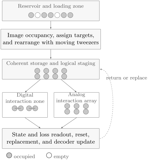
A conceptual zone-based neutral-atom dataflow. Static tweezer arrays provide storage, while dynamic tweezers rearrange loaded atoms and route selected qubits. Digital Rydberg gates use scheduled pairs; analog operation uses a programmed many-body geometry. Readout, reset, and replacement remove entropy before atoms or logical blocks return to storage.

This separation can protect stored data from resonant light and concentrate expensive addressing resources. It also turns movement into part of the instruction set. For a move of duration $T_m$, the relevant record includes survival, coherence, motional excitation, phase accumulation, handoff error, and path conflicts. A transport fidelity inferred from a return experiment may not separately identify those mechanisms.

Let one repeated logical cycle contain routing, gates, measurement, reset, and classical decision. A serial latency model is

$$\begin{aligned} T_{\mathrm{cycle}} &= T_{\mathrm{route}} +T_{\mathrm{gate}} \\ &\quad+ T_{\mathrm{read}} +T_{\mathrm{reset}} \\ &\quad+ T_{\mathrm{classical}}. \end{aligned}$$

With separate zones, some terms can overlap across batches. The asymptotic cadence is then bounded below by the slowest occupied pipeline stage, but route conflicts, finite reservoirs, dynamic branches, and feedback barriers can prevent ideal overlap.

Zone-based designs also permit qubit reuse: a measured atom can be reset and returned, or a lost atom can be replaced by one from the reservoir. This is not automatic fault tolerance. Reuse must preserve the logical state carried by the remaining atoms, report the replacement location to the decoder, and avoid contamination from measurement light or transport.

Measurement, Reset, Loss, and Erasure

Presence and internal state are different observables

Fluorescence imaging readily answers whether an atom occupies a site. Reading the qubit additionally requires a state-dependent mapping, such as bright/dark fluorescence, shelving, blow-away followed by presence detection, or spin-to-position conversion. The outcome alphabet may be

$$y\in\{0,1,\varnothing\},$$

where $\varnothing$ denotes detected absence. A three-outcome confusion matrix is therefore more informative than a single assignment fidelity:

$$M_{y|x}=P(y\mid x), \qquad x\in\{0,1,\mathrm{lost}\}.$$

A destructive method can have excellent terminal readout while being unsuitable for repeated syndrome extraction. Mid-circuit operation asks for low disturbance to spectators, low atom loss, controlled reset, and bounded latency in addition to classification accuracy.

Loss can be useful information

Atom loss leaves the computational Hilbert space. If it is detected with a known location, the event is an erasure rather than an unlocated error. Suppose a mechanism causes loss with probability $p_{\ell}$ and the experiment identifies it with efficiency $\eta_e$. In a simple bookkeeping model,

$$\begin{aligned} p_{\mathrm{located}} &=\eta_e p_{\ell}, \\ p_{\mathrm{unlocated}} &=(1-\eta_e)p_{\ell}. \end{aligned}$$

False erasure flags, delayed detection, and faults occurring after the last check must be added. The same physical process can therefore produce a mixture of located erasures, unlocated leakage, and ordinary Pauli error.

Alkaline-earth-like atoms offer additional manifolds that can convert some decay or leakage events into detectable population outside the qubit pair. This erasure conversion changes the information supplied to the decoder; it does not erase the physical fault. Its benefit depends on conversion efficiency, flag fidelity, correlations, reset cost, and the code’s response to located faults.

Large arrays amplify small loss probabilities

If each of $N$ active atoms independently survives one cycle with probability $s$, then

$$P_{\mathrm{no\ loss}}(K) = s^{NK}$$

is the probability that no atom is lost in $K$ cycles. This exponential is a warning against postselecting only shots in which every atom survives. At scale, a useful architecture must detect, tolerate, replace, or correct loss rather than demand that it never happen.

Independence is only a baseline. Vacuum events may be approximately local, whereas laser excursions, trap-power changes, image-light errors, or path collisions can produce correlated loss. Reporting only average survival hides the distinction.

Analog Quantum Simulation

From geometry to an interacting spin model

With $\lvert0\rangle$ treated as an unexcited state and $\lvert1\rangle$ as a Rydberg-coupled state, global coherent driving can realize a soft-constraint Ising-type Hamiltonian

$$\begin{aligned} \frac{H}{\hbar} &= \frac{\Omega(t)}{2}\sum_i\sigma_i^x -\Delta(t)\sum_i n_i \\ &\quad+ \sum_{i<j} \frac{V_{ij}}{\hbar}n_i n_j, \qquad n_i=\frac{1+\sigma_i^z}{2}. \end{aligned}$$

The sign in $n_i=(1+\sigma_i^z)/2$ is a convention; some authors exchange the eigenvalue assigned to the excited state. Geometry sets $R_{ij}$, the selected Rydberg state and fields set $V_{ij}$, and laser waveforms set $\Omega(t)$ and $\Delta(t)$. In the strong-blockade limit, nearby simultaneous excitations are energetically suppressed, leading to constrained models such as the PXP model. The canonical derivation belongs in Rydberg Blockade.

Analog is not gate-based digital computation

An analog experiment programs a Hamiltonian and observes its evolution. A digital experiment compiles an abstract circuit into calibrated gates. The same apparatus can support both, but evidence does not transfer automatically:

Question	Digital mode	Analog mode
programmed object	gate sequence	geometry and time-dependent Hamiltonian
primary calibration	process or gate instruction	$\Omega_i$, $\Delta_i$, $V_{ij}$, geometry
dominant comparison	circuit or logical output	observables, correlations, phase structure, dynamics
validation	randomized circuits, tomography, logical tests	limits, symmetries, size scaling, independent methods
typical failure	coherent gate accumulation, leakage, routing	Hamiltonian mismatch, inhomogeneity, state-preparation bias

Hundreds of interacting atoms in an analog simulation do not imply a universal hundreds-qubit digital computer. Conversely, gate benchmarks do not establish that a many-body Hamiltonian is known accurately across every pair.

What must be validated

A defensible analog result reports:

• the realized geometry and position uncertainty;
• spatial maps of Rabi frequency, detuning, and relevant pair interactions;
• preparation, detection, loss, and postselection procedures;
• finite ramp rates, temperature, decoherence, and total evolution time;
• observables chosen before data interpretation where possible;
• checks against exactly solvable limits, small-system numerics, symmetries, conservation laws, and alternative ramps or geometries;
• uncertainty from both measurement and Hamiltonian calibration.

What Is Quantum Simulation? develops the platform-neutral distinction among analog, digital, and hybrid simulation and the corresponding validation ladder.

Noise and Error Mechanisms

Neutral-atom errors are not captured by one coherence time or one average gate fidelity.

Mechanism	Physical origin	Observable signature	Architectural response
storage dephasing	magnetic noise, differential light shifts, motion through inhomogeneous traps	Ramsey decay, spatially varying phase	clock states, magic conditions, echo, trap calibration
population relaxation	optical pumping, Raman scattering, blackbody or environmental coupling	state-dependent $T_1$, leakage	detuning, filtering, state choice, leakage checks
trap loss	background collisions, heating, shallow traps, imaging and transport	empty site, survival decay	better vacuum, cooling, reservoirs, erasure-aware decoding
motional error	finite temperature, acceleration, trap handoff, recoil	contrast or gate error versus temperature and trajectory	cooling, smooth transport, composite pulses
Rydberg decay	spontaneous and blackbody-driven transitions	loss, leakage, dephasing during gates	faster optimized pulses, state choice, erasure conversion
finite blockade	interaction shift too small or inhomogeneous	double excitation, coherent phase error	geometry, pulse shaping, pair calibration
laser noise	phase, frequency, intensity, pointing, wavefront	coherent rotation error, drift, site dependence	stabilization, common-mode design, local monitors
addressing crosstalk	finite beam waist, shared AOD tones, scattered light	spectator rotations or Stark shifts	cancellation, spacing, scheduling, calibration in parallel context
electric-field sensitivity	dc and ac fields, surface charge, ion production	Rydberg detuning and pair-state drift	electrodes, compensation, shielding, frequent spectroscopy
readout backaction	resonant photons, imperfect shelving, detector confusion	spectator error, loss, false erasure	spatial zones, hiding, non-destructive mapping, decoder model
correlated faults	common lasers, trap power, camera, waveform or vacuum events	spatial and temporal clusters	correlation-aware diagnostics, interlocks, code-aware scheduling

Memory coherence is conditional

An echo or dynamical-decoupling time is measured under a specific pulse train, trap depth, temperature, and field environment. It is not necessarily the available algorithmic idle time. During computation, atoms may move, traps may change depth, Rydberg beams may illuminate spectators, and phase frames may be updated. Useful memory benchmarks reproduce those conditions.

Loss and leakage need time stamps

Finding an empty site at final readout does not reveal when the atom left. A decoder may need to know whether the loss occurred before or after a given entangling gate. Intermediate presence checks, circuit cancellation rules, and probabilistic loss-time models can supply this information. The decoder and hardware schedule are therefore coupled.

Parallel operation can reveal new errors

A high-fidelity isolated pair gate may degrade in a dense layer because of shared optical power, AOD intermodulation, spectator interactions, wavefront variation, or common laser transients. Characterization should therefore include the intended simultaneous patterns and not only one pair at a time.

Infrastructure and Control

Vacuum and atom source

Vacuum lifetime sets a basic hazard rate for loss. Large arrays magnify even a small per-atom rate, so loading architecture, differential pumping, source contamination, and local pressure matter. A long single-atom lifetime should be translated into array-level no-loss probabilities at the relevant cycle duration.

Cryogenic and Vacuum Infrastructure develops that translation from local gas loads and species through collision hazards, whole-array survival, diagnostics, source cycles, and availability.

Repeated or continuous operation also needs an atom supply that does not disturb stored qubits. A reservoir can be spatially separated from storage, but cooling and imaging light, magnetic transients, and moving traps still need isolation and scheduling.

Optical system

A neutral-atom processor may require trapping, cooling, imaging, pumping, Raman, clock, Rydberg, shelving, and repumping wavelengths. The high-numerical- aperture objective must combine field of view, resolution, wavefront quality, chromatic performance, and collection efficiency. Scaling site count can stress laser power and aberration correction; scaling parallel control can stress modulator bandwidth, tone count, and beam steering.

The optical system should be described as a calibrated transfer function from commanded waveform to field at each atom. Camera images alone do not capture phase, polarization, or fast intensity transients.

Electric and magnetic fields

Rydberg levels have large polarizabilities and can be sensitive probes of stray electric fields. Photocharging, ions generated during operation, electrode drift, and nearby surfaces can shift the resonance. Bias magnetic fields define quantization and separate Zeeman components but also create spatial detuning if gradients are uncontrolled. Pair-state spectroscopy and field compensation belong in the routine calibration graph.

Timing, computation, and provenance

Static holograms, moving-tweezer trajectories, Raman and Rydberg pulses, camera exposures, classifier execution, routing, and decoder decisions must share a timing model. A useful control stack records:

• the compiled atom-to-logical-qubit assignment;
• every trajectory and zone occupancy interval;
• waveform and calibration versions;
• images, classifier thresholds, and erasure flags;
• branch decisions and cancelled gates after loss;
• environmental monitors and drift interventions;
• raw data sufficient to reconstruct reported metrics.

As arrays grow, calibration is not a flat list. Trap depth affects temperature and light shift; those affect Rabi and Rydberg detuning; geometry affects interaction; all of them affect gate performance. Control, Readout, and Calibration develops dependency-aware calibration and validation.

Throughput and Scheduling

Fast microscopic gates do not guarantee fast experiments. A shot can include

$$\begin{aligned} T_{\mathrm{shot}} &= T_{\mathrm{load}} +T_{\mathrm{image}} \\ &\quad+ T_{\mathrm{rearrange}} +T_{\mathrm{cool}} \\ &\quad+ T_{\mathrm{prepare}} +T_{\mathrm{circuit}} \\ &\quad+ T_{\mathrm{read}} +T_{\mathrm{classical}}. \end{aligned}$$

Loading and initial rearrangement can dominate a one-shot laboratory cycle. Persistent reservoirs and mid-circuit replacement can amortize those costs, but introduce pipeline and contamination constraints. Reporting gate duration without shot cadence, duty cycle, and accepted-shot fraction cannot predict time to solution.

For a logical circuit, movement can reduce gate depth by enabling nonlocal pairings, yet increase wall-clock time. A rough compiled cost is

$$C_{\mathrm{compiled}} = \alpha D_g +\beta D_m +\gamma N_h +\delta N_r,$$

where $D_g$ is gate depth, $D_m$ movement depth, $N_h$ the number of handoffs, and $N_r$ the number of readout/reset barriers. Coefficients should come from measured latency and error, and may depend on which operations overlap.

Useful throughput reports include:

• initialized active qubits per second;
• parallel one- and two-qubit operation width;
• circuit shots per second at a stated depth;
• accepted shots per second after declared filters;
• syndrome rounds per second and decoder latency;
• useful logical operations per second at a stated logical error rate;
• reservoir depletion and replenishment rates.

Error-Correction Fit

Architectural opportunities

Neutral-atom arrays offer several features relevant to error correction:

• atoms are naturally uniform, so fabrication spread does not set their bare internal spectrum;
• arrays can be rearranged into code-specific geometries;
• coherent movement can provide nonlocal pairings or transversal operations without long swap chains;
• loss can often be detected directly and supplied as erasure information;
• readout, reset, and reservoir zones can remove entropy and replenish atoms;
• blockade can support parallel controlled phases and some multiqubit operations.

These features do not select a unique code. Surface codes favor repeated local checks and strict measurement cadence. Quantum LDPC and transversal-gate schemes may exploit longer-range transport or block movement. The right choice depends on the measured movement, gate, loss, readout, reset, and correlation model, not connectivity alone.

Repeated correction is the decisive test

A logical state preparation or postselected logical circuit is evidence of encoding, not yet of sustained error correction. Stronger demonstrations ask whether increasing code resources or repeated syndrome rounds suppresses a logical error under a stated decoder and acceptance policy. Claims should separate:

• error detection from active or frame-based correction;
• one round from repeated rounds;
• postselected from unconditional performance;
• physical-qubit count from active and logical-qubit counts;
• a memory experiment from universal logical operations;
• below-threshold scaling in a tested finite regime from a complete fault-tolerant computer.

Loss-aware decoding is especially important. If a loss is detected only at the end, its possible time locations must be propagated through the circuit. If a qubit is replaced, the reset and reinsertion operation belongs in the circuit-level error model.

Dated evidence through August 2026

The following entries are milestones, not a leaderboard. Protocols and scopes differ.

Date	Demonstrated object	What the evidence supports	What it does not establish
2022	coherent transport of entangled atom arrays	dynamic geometry can preserve entanglement and enable programmable pairings	arbitrary transport schedules at large fault-tolerant scale
2023	parallel controlled-Z gates on up to 60 atoms with about 99.5% reported fidelity	high-fidelity Rydberg gates can operate in parallel under the tested protocol	the same fidelity on every pair or at arbitrary array size
2024	reconfigurable logical processor with up to 48 logical qubits on 280 atoms	logical encoding, transversal operations, movement, and logical algorithms can be integrated	sustained large-distance fault-tolerant computation
2025	more than 6,100 coherent atomic qubits in roughly 12,000 tweezers	large-scale storage, imaging, global control, and coherent transport	6,100 simultaneous entangling qubits or a 6,100-qubit logical processor
2025	continuous operation of a coherent system with more than 3,000 qubits for over two hours	replenishment can maintain a large operating array while preserving qubit coherence	one fixed 3,000-qubit state cohering for two hours
2026	up to 448 atoms in a zone-based logical architecture	four-round below-threshold characterization, logical operations, mid-circuit reuse, and entropy-removal ingredients	a general-purpose, application-scale fault-tolerant computer
2026	logical qubits and erasure conversion with metastable neutral atoms	manifold mapping can turn selected faults into decoder-visible erasures	perfect conversion of all dominant faults or universal fault tolerance

The 2026 fault-tolerant-architecture paper reports a factor $2.14(13)$ below threshold in a specific four-round characterization circuit, alongside transversal, lattice-surgery, teleportation, and reuse experiments. A published correction belongs to the citation record. The durable conclusion is that several key mechanisms have now been combined experimentally. The finite device, finite code distances, decoder assumptions, circuit families, and measured error model remain essential qualifiers.

For a fuller, frequently reviewed assessment of current claims and open problems, see Rydberg Array Frontiers.

Advantages and Bottlenecks

Durable advantages

1. Atomic reproducibility. Qubit transition variation is set mainly by the environment rather than lithographic device variation.
2. Reconfigurable geometry. Tweezer positions can be adapted to a model, circuit layer, or code block.
3. Separated storage and interaction. Long-lived internal states can store information while Rydberg states mediate fast temporary coupling.
4. Large optical field of view. Thousands of sites and atoms can be created without fabricating one nonlinear element per qubit.
5. Direct atom-resolved observation. Presence, state, and loss can be inferred spatially.
6. Digital and analog operation. One platform can implement calibrated gates or many-body Hamiltonians.
7. Erasure opportunities. Some loss and leakage events can be located or converted into detectable manifolds.

Persistent bottlenecks

1. Optical complexity. Many stable wavelengths, wavefronts, phases, polarizations, and steering channels must coexist over a large field.
2. Stochastic loading and loss. Rearrangement and reservoirs are part of routine operation, not optional setup details.
3. Rydberg lifetime and sensitivity. Strong interaction comes with decay, blackbody coupling, multilevel structure, and electric-field sensitivity.
4. Parallel calibration. Pair gates that work separately can interfere through blockade, beams, modulators, or shared power.
5. Measurement isolation. Resonant fluorescence is powerful but can heat, depump, or dephase nearby data.
6. Movement overhead. Reconfigurability buys reachability at a cost in latency, handoffs, heating, loss, and scheduling.
7. Array-level tail risk. Small per-atom loss or calibration outliers become common somewhere in a large machine.
8. Evidence translation. Storage scale, analog scale, parallel-gate scale, and logical scale are not interchangeable.

Worked Architecture Audit

Consider a notional zone-based processor with 320 storage sites, 256 active data and ancilla atoms, a reservoir of 64 atoms, 32 simultaneous interaction pairs, and per-active-atom survival $s=0.9995$ per repeated cycle.

1. Check array-level survival

Under the independent model, the probability that all 256 active atoms survive one cycle is

$$P_1 = (0.9995)^{256} \approx 0.880.$$

After 100 cycles, demanding that every atom survive throughout gives

$$\begin{aligned} P_{100} &= (0.9995)^{25600} \\ &\approx e^{-12.8} \approx 2.8\times10^{-6}. \end{aligned}$$

The architecture cannot scale by accepting only trajectories with no loss. It needs timely loss detection, erasure-aware decoding, replacement, or logical tolerance.

2. Separate gate width from qubit count

The processor has 256 active atoms but only 32 interaction pairs per gate layer. A circuit layer containing 96 compatible two-qubit gates therefore requires at least

$$\left\lceil\frac{96}{32}\right\rceil=3$$

gate batches before routing conflicts or local corrections are included. The active-qubit count alone would miss this factor.

3. Budget a pipelined correction cycle

Suppose a batch requires $180\,\mu\mathrm{s}$ of movement, $1.5\,\mu\mathrm{s}$ of Rydberg pulses and phase corrections, $250\,\mu\mathrm{s}$ of readout/reset, and $35\,\mu\mathrm{s}$ of classical processing. If movement for the next batch can overlap readout of the previous batch, an optimistic steady-state cadence is bounded by

$$\begin{aligned} T_{\mathrm{batch}} &\ge \max(180,285)\,\mu\mathrm{s} \\ &\quad+ 1.5\,\mu\mathrm{s} \\ &= 286.5\,\mu\mathrm{s}. \end{aligned}$$

Three batches then require at least $859.5\,\mu\mathrm{s}$ in steady state, plus pipeline fill, drain, and feedback barriers. The microscopic gate pulse is not the dominant latency.

4. Test reservoir sufficiency

The expected number of losses per cycle is

$$\mathbb E[L] = 256(1-s) = 0.128.$$

A 64-atom reservoir is therefore about 500 expected cycles of replacement in this simple mean-value calculation. That statement is not a reliability guarantee: losses fluctuate, replacement can fail, the reservoir itself can lose atoms, and reload operations may occur in fixed batches. A full design uses the loss distribution and replenishment cadence, not only its mean.

Audit conclusion

The most urgent improvements are not inferred from the qubit count. One must measure which loss events are located, how quickly replacement occurs, whether the decoder uses loss timing, which 32-pair patterns are legal, and whether movement and readout truly overlap. The architecture is defined by this workflow, not by the largest number in its specification.

Evidence and Reporting Ledger

For a reproducible neutral-atom claim, record the following:

Claim class	Minimum evidence
array size	trap sites, loaded atoms, encoded/calibrated/active subsets, spatial map
loading	per-site and array distribution, correlations, image classifier, rearrangement yield
storage	sequence, trap condition, active subset, $T_1$, $T_2^*$, echo or decoupled $T_2$
one-qubit control	global/local distinction, gate set, leakage, spectator effect, parallel pattern
Rydberg gate	states, geometry, pulse, simultaneous pairs, SPAM treatment, loss treatment, uncertainty
connectivity	direct or routed edges, pair calibration, parallel width, movement and handoff cost
analog simulation	Hamiltonian map, geometry, calibration uncertainty, validation and postselection
readout	full confusion matrix, loss discrimination, spectator disturbance, duration, reset
transport	distance, trajectory, atom number, coherence, survival, handoffs, temperature
error correction	code, physical and logical counts, rounds, decoder, acceptance, correlations, scaling test
throughput	full shot or syndrome cadence, duty cycle, accepted-shot rate, classical latency
dated record	device, protocol, uncertainty, exact date, source, correction or erratum status

Common Mistakes

Treating every trap site as a qubit

An empty optical minimum is not an atom; a loaded atom is not necessarily encoded, calibrated, active, entangled, or logical. Report the complete count chain.

Equating array size with computational width

Large storage arrays can demonstrate coherence, imaging, and transport without running entangling gates on every atom. State the active subset and parallel gate width.

Calling rearrangement deterministic

Rearrangement can produce a nearly defect-free target from stochastic loading, conditional on enough atoms, correct images, feasible routes, and successful transport. It does not make the microscopic loading process deterministic.

Treating the blockade radius as a hard cutoff

$R_b$ is a comparison scale. Residual spectator interactions persist outside it, and interaction strength varies inside it.

Using one pair-gate number for an entire array

Gate performance depends on pair geometry, site, time, and simultaneous pulse pattern. An isolated best pair is not an array-wide specification.

Ignoring loss in fidelity estimates

Postselecting lost atoms can make conditional state fidelity look high while lowering unconditional success. Report conditional quality, loss probability, and accepted-shot rate separately.

Calling detected loss harmless

An erasure is easier for many codes because its location is known, but it is still a fault. Detection efficiency, timing ambiguity, false flags, and reset must enter the decoder model.

Mixing analog and digital evidence

An analog many-body experiment and a digital circuit benchmark validate different programmed objects. Do not infer one from the other.

Treating long continuous operation as one long coherent state

A replenished processor can operate coherently for hours while individual subarrays are replaced. Describe the replacement schedule and the coherence preserved across it.

Calling a finite demonstration a completed fault-tolerant computer

Below-threshold behavior, logical gates, teleportation, reuse, and erasure conversion are major ingredients. Their demonstration in finite protocols does not yet establish application-scale universal fault-tolerant operation.

Exercises

1. Quantify the loading problem

One hundred target tweezers load independently with probability $p=0.75$. Find the probability that all target sites are filled without rearrangement. Explain why an average of 75 atoms is not enough to characterize preparation.

Solution

The full-array probability is

$$P_{\mathrm{full}} =(0.75)^{100} \approx 3.21\times10^{-13}.$$

The mean occupancy is 75, but a quantum circuit usually requires atoms at specific sites. The occupancy distribution, correlations, and spatial pattern matter. Rearrangement uses excess source sites to convert the random pattern into a target pattern, conditional on having enough correctly identified atoms and moving them successfully.

2. Size a source array

A target requires 200 atoms. Source sites load independently with probability $0.60$. What is the smallest integer $M$ for which the mean number loaded is at least 240? Why does this not guarantee a 200-atom target?

Solution

The mean is $0.60M$, so

$$0.60M\ge240 \quad\Longrightarrow\quad M\ge400.$$

Thus the smallest integer by the stated mean criterion is $M=400$. The actual number is a random variable with standard deviation

$$\begin{aligned} \sqrt{Mp(1-p)} &= \sqrt{400(0.60)(0.40)} \\ &= \sqrt{96} \approx9.80. \end{aligned}$$

The mean exceeds 200 by about four standard deviations, but success also depends on correlated loading, image errors, route feasibility, movement loss, and target verification. A reliability requirement should use a tail probability and measured nonidealities, not only the mean.

3. Estimate finite-blockade leakage

A gate uses $\Omega/2\pi=4\,\mathrm{MHz}$ and a calibrated blockade shift $B/2\pi=40\,\mathrm{MHz}$. Estimate $(\Omega/B)^2$. What is omitted?

Solution

The ratio is independent of whether both quantities are quoted as angular or ordinary frequencies, provided the convention is consistent:

$$\left(\frac{\Omega}{B}\right)^2 = \left(\frac{4}{40}\right)^2 = 10^{-2}.$$

This one-percent scale is only the elementary finite-blockade estimate. It omits pulse-shape coefficients, coherent phase error, decay, intermediate- state scattering, Doppler and position effects, multilevel pair states, laser noise, preparation, measurement, and loss classification.

4. Compute a Rydberg-decay floor

During a $1.0\,\mu\mathrm{s}$ gate, the total integrated Rydberg population is

$$\int_0^{T_g}P_r(t)\,dt=0.45\,\mu\mathrm{s}.$$

For effective lifetime $\tau_r=150\,\mu\mathrm{s}$, estimate the decay probability to first order.

Solution

For a small probability,

$$p_{\mathrm{decay}} \approx \frac{0.45\,\mu\mathrm{s}}{150\,\mu\mathrm{s}} = 3.0\times10^{-3}.$$

The estimate says nothing about whether decay produces a Pauli error, leakage, loss, or a detected erasure. Those branches have different consequences for a logical circuit.

5. Compare target and spectator interactions

Under an isotropic $C_6/R^6$ approximation, a target pair is separated by $5\,\mu\mathrm{m}$ and a spectator is $10\,\mu\mathrm{m}$ from one member. Find the magnitude ratio $|V_{\mathrm{spectator}}/V_{\mathrm{target}}|$.

Solution

The coefficient cancels:

$$\begin{aligned} \left| \frac{V_{\mathrm{spectator}}}{V_{\mathrm{target}}} \right| &= \left(\frac{5}{10}\right)^6 \\ &= \frac{1}{64} \approx1.56\times10^{-2}. \end{aligned}$$

The spectator interaction is not zero. Whether it is acceptable depends on the pulse, detuning, duration, allowed coherent phase, angular dependence, and other nearby atoms.

6. Separate reachability from parallel width

A 48-atom array can route any selected pair to an interaction zone. The zone supports at most eight simultaneous pairs. A circuit layer requests 20 disjoint pair gates. Give the abstract pair reachability count and a lower bound on the number of batches.

Solution

If every pair is reachable, the pair graph has

$$\binom{48}{2} = 1128$$

edges. The 20 requested gates require at least

$$\left\lceil\frac{20}{8}\right\rceil =3$$

batches. Route conflicts, pair-dependent calibration, and local corrections can increase the actual number. The 1,128 reachable edges do not describe simultaneous connectivity.

7. Audit survival scaling

For $N=500$ active atoms and per-cycle survival $s=0.9998$, find the probability of no loss in one cycle and in 50 cycles under independence.

Solution

For one cycle,

$$P_1 =(0.9998)^{500} \approx e^{-0.10} \approx0.905.$$

For 50 cycles,

$$\begin{aligned} P_{50} &=(0.9998)^{25000} \\ &\approx e^{-5.00} \\ &\approx6.74\times10^{-3}. \end{aligned}$$

Thus excellent per-atom survival is compatible with frequent array-level loss. Detected erasures, replacement, and logical tolerance become system requirements.

8. Expand the analog interaction term

Using $n_i=(1+\sigma_i^z)/2$, expand $V_{ij}n_i n_j$. Identify the constant, single-spin, and Ising-coupling pieces.

Solution

Direct expansion gives

$$V_{ij}n_i n_j = \frac{V_{ij}}{4} \left( 1+\sigma_i^z+\sigma_j^z +\sigma_i^z\sigma_j^z \right).$$

The first term is a constant energy offset. The middle terms contribute local longitudinal fields when summed over pairs. The last is an Ising coupling of strength $V_{ij}/4$ under this Pauli convention. Dropping the constant is safe for dynamics, but the induced local fields must be combined consistently with the detuning term.

9. Split located and unlocated loss

A gate has loss probability $p_{\ell}=3.0\times10^{-3}$. The loss-detection efficiency is $\eta_e=0.92$, and false erasure flags occur with probability $2.0\times10^{-4}$ per gate. Compute the simple located and missed-loss probabilities, and state why the false flag is separate.

Solution

The located part is

$$\begin{aligned} p_{\mathrm{located}} &=(0.92)(3.0\times10^{-3}) \\ &=2.76\times10^{-3}, \end{aligned}$$

and the missed part is

$$\begin{aligned} p_{\mathrm{unlocated}} &=(0.08)(3.0\times10^{-3}) \\ &=2.4\times10^{-4}. \end{aligned}$$

The $2.0\times10^{-4}$ false-flag probability occurs when the decoder is told an erasure happened even though the specified loss did not. It is not part of $p_{\ell}$ and must be represented as a separate observation error. Correlated flags and timing ambiguity would require a richer model.

10. Audit a scale claim

A report states: “The platform operates 6,100 qubits and therefore supports 3,050 parallel two-qubit gates.” List the evidence needed before accepting the conclusion.

Solution

First ask what 6,100 counts: loaded atoms, coherently encoded atoms, calibrated qubits, active qubits, or atoms participating in a circuit. Then request the Rydberg interaction region, selected pair states, pair separations and orientations, local and global addressing resources, optical-power budget, legal simultaneous patterns, blockade conflicts, spectator errors, and gate fidelity under full parallel load.

Also ask whether atoms must be routed, how many moving traps and interaction zones exist, and the movement, handoff, and scheduling cost. Finally require the benchmark protocol, uncertainty, SPAM and loss treatment, postselection, date, and active pair map. The arithmetic bound $\lfloor6100/2\rfloor=3050$ only counts disjoint pairs; it does not demonstrate that hardware can execute all of them simultaneously.

References

1. M. Saffman, T. G. Walker, and K. Mølmer, “Quantum information with Rydberg atoms,” Reviews of Modern Physics 82, 2313–2363 (2010), doi:10.1103/RevModPhys.82.2313.
2. D. Jaksch et al., “Fast quantum gates for neutral atoms,” Physical Review Letters 85, 2208–2211 (2000), doi:10.1103/PhysRevLett.85.2208.
3. M. Saffman, “Quantum computing with atomic qubits and Rydberg interactions: Progress and challenges,” Journal of Physics B 49, 202001 (2016), doi:10.1088/0953-4075/49/20/202001.
4. M. Morgado and S. Whitlock, “Quantum simulation and computing with Rydberg-interacting qubits,” AVS Quantum Science 3, 023501 (2021), doi:10.1116/5.0036562.
5. A. M. Kaufman and K.-K. Ni, “Quantum science with optical tweezer arrays of ultracold atoms and molecules,” Nature Physics 17, 1324–1333 (2021), doi:10.1038/s41567-021-01357-2.
6. H. Bernien et al., “Probing many-body dynamics on a 51-atom quantum simulator,” Nature 551, 579–584 (2017), doi:10.1038/nature24622.
7. H. Levine et al., “Parallel implementation of high-fidelity multiqubit gates with neutral atoms,” Physical Review Letters 123, 170503 (2019), doi:10.1103/PhysRevLett.123.170503.
8. A. Browaeys and T. Lahaye, “Many-body physics with individually controlled Rydberg atoms,” Nature Physics 16, 132–142 (2020), doi:10.1038/s41567-019-0733-z.
9. P. Scholl et al., “Quantum simulation of 2D antiferromagnets with hundreds of Rydberg atoms,” Nature 595, 233–238 (2021), doi:10.1038/s41586-021-03585-1.
10. S. Ebadi et al., “Quantum phases of matter on a 256-atom programmable quantum simulator,” Nature 595, 227–232 (2021), doi:10.1038/s41586-021-03582-4.
11. A. Omran et al., “Generation and manipulation of Schrödinger cat states in Rydberg atom arrays,” Science 365, 570–574 (2019), doi:10.1126/science.aax9743.
12. D. Bluvstein et al., “A quantum processor based on coherent transport of entangled atom arrays,” Nature 604, 451–456 (2022), doi:10.1038/s41586-022-04592-6.
13. H. Levine et al., “Dispersive optical systems for scalable Raman driving of hyperfine qubits,” Physical Review A 105, 032618 (2022), doi:10.1103/PhysRevA.105.032618.
14. H. Evered et al., “High-fidelity parallel entangling gates on a neutral-atom quantum computer,” Nature 622, 268–272 (2023), doi:10.1038/s41586-023-06481-y.
15. P. Scholl et al., “Erasure conversion in a high-fidelity Rydberg quantum simulator,” Nature 622, 273–278 (2023), doi:10.1038/s41586-023-06516-4.
16. D. Bluvstein et al., “Logical quantum processor based on reconfigurable atom arrays,” Nature 626, 58–65 (2024), doi:10.1038/s41586-023-06927-3.
17. H. J. Manetsch et al., “A tweezer array with 6,100 highly coherent atomic qubits,” Nature 647, 60–67 (2025), doi:10.1038/s41586-025-09641-4.
18. C.-M. Chiu et al., “Continuous operation of a coherent 3,000-qubit system,” Nature 646, 1075–1080 (2025), doi:10.1038/s41586-025-09596-6.
19. R. Sales Rodriguez et al., “Experimental magic state distillation for fault-tolerant quantum computing,” Nature 645, 620–625 (2025), doi:10.1038/s41586-025-09367-3.
20. D. Bluvstein et al., “A fault-tolerant neutral-atom architecture for universal quantum computation,” Nature 649, 39–46 (2026), doi:10.1038/s41586-025-09848-5; correction, doi:10.1038/s41586-026-10108-3.
21. S. Zhang et al., “Logical qubits with erasure conversion using metastable neutral atoms,” Nature Physics 22, 910–916 (2026), doi:10.1038/s41567-026-03309-0.
22. A. Senoo et al., “High-fidelity entanglement and state-manifold mapping with neutral atoms,” Nature Physics 22, 903–909 (2026), doi:10.1038/s41567-026-03258-8.
23. M. A. Norcia et al., “Mid-circuit qubit measurement and rearrangement in a $^{171}\mathrm{Yb}$ atomic array,” Physical Review X 13, 041034 (2023), doi:10.1103/PhysRevX.13.041034.
24. M. A. Norcia et al., “Seconds-scale coherence on an optical clock transition in a tweezer array,” Science 366, 93–97 (2019), doi:10.1126/science.aay0644.

Further Connections

• Magic State Distillation gives the protocol and evidence context for the 2025 neutral-atom logical 5-to-1 demonstration, including what it does and does not establish about a sustained factory.
• Lattice Surgery develops the protected parity-measurement protocol and places neutral-atom ancilla-mediated parity demonstrations in their code-distance and fault-tolerance context.
• Hardware Overview compares neutral atoms with superconducting circuits, trapped ions, photons, semiconductor spins, bosonic modes, and topological proposals under one system contract.
• Metrics for Quantum Hardware defines storage, operation, leakage, loss, crosstalk, connectivity, throughput, logical, and workload metrics.
• Control, Readout, and Calibration develops waveform validation, detector inference, calibration dependencies, drift monitoring, and feedback.
• Cryogenic and Vacuum Infrastructure develops the local-pressure, gas-load, collision, whole-array loss, diagnostics, recovery, and availability ledger behind neutral-atom operation.
• Materials and Fabrication Interface treats chamber surfaces, electrodes, coatings, windows, optical assemblies, and process variation as apparatus-level sources whose distributions constrain field control, optical uniformity, reliability, and array acceptance.
• Optical Tweezers provides the canonical trap, loading, imaging, cooling, rearrangement, and transport physics.
• Rydberg Atoms develops state selection, excitation, fields, trapping, lifetime, detection, and pair calibration.
• Rydberg Blockade derives blockade, collective states, finite-interaction corrections, entangling protocols, and constrained dynamics.
• Neutral Atoms in Open Systems develops scattering, imaging backaction, dephasing, Rydberg decay, and loss models.
• Rydberg Array Frontiers maintains the dated assessment of analog simulation, optimization, logical processing, and fault-tolerance claims.
• Analog Quantum Simulation derives the general target–device mapping and the Rydberg-to-Ising reduction, including induced longitudinal fields, interaction tails, leakage, and validation requirements.
• What Is Quantum Simulation? distinguishes analog, digital, and hybrid simulation and explains validation strategies.
• Surface Code supplies one canonical framework for repeated stabilizer extraction, decoding, logical operations, and overhead.