Continuous-Variable Platforms

A continuous-variable platform processes quantum information in observables with continuous spectra, most often the field quadratures of optical or microwave bosonic modes. Its native resources are squeezed states, interferometers, phase-space displacements, homodyne or heterodyne measurements, and classical feedforward. These operations are deterministic and high bandwidth in several mature technologies.

That description is only the Gaussian backbone. Gaussian states, Gaussian operations, and Gaussian measurements by themselves do not provide universal quantum computation, nor do they generally evade efficient classical simulation. A universal or fault-tolerant architecture must introduce a well-characterized non-Gaussian resource, such as photon counting, photon-conditioned state preparation, a cubic-phase-like state, or a finite-energy grid state. It must then preserve that scarce resource through loss, mode mismatch, finite squeezing, phase noise, detection, and feedforward.

Continuous-variable hardware should therefore be judged as a complete source-to-output system. A large number of modes can establish multiplexing and entanglement capability without establishing universality. A hard sampling experiment can demonstrate a computational task without demonstrating error-corrected logical gates. A non-Gaussian state source can be an essential module without yet being a fault-tolerant processor.

Purpose and Canonical Scope

This page owns the hardware and architecture layer for continuous-variable quantum information:

• optical and microwave mode definitions and physical implementations;
• Gaussian state generation, mode mixing, measurement, and feedforward;
• where non-Gaussianity enters and what hardware it costs;
• time-, frequency-, and spatial-mode connectivity;
• optical loss, thermal noise, phase jitter, mode mismatch, detector noise, finite squeezing, and probabilistic resource yield;
• fair platform metrics and end-to-end resource accounting;
• experimental evidence and claim boundaries through 10 August 2026.

Continuous-Variable Quantum Computation owns the device-independent model semantics: mode registers, Gaussian and non-Gaussian computational operations, continuous measurement and feedforward, CV-cluster logic, output decoding, approximation metrics, and abstract resource accounting. This page retains physical optical and microwave architectures, resource generation, loss, detectors, timing, calibration, and experimental evidence.

Continuous-Variable Systems owns the Hilbert-space foundations, quadrature eigenstates, multimode kinematics, and the continuous-variable form of entanglement. Gaussian States and Wigner Functions owns phase-space quasiprobabilities and covariance-matrix mathematics. Gaussian Channels owns the channel classification. Squeezed Light and Homodyne and Heterodyne Detection develop the corresponding quantum-optical mechanisms and detector theory.

Bosonic Qubits owns finite-dimensional logical encodings in oscillators, including the hardware implications of cat, binomial, and grid codes. Cat Codes owns coherent-component encodings and their loss-sector and bias conventions. GKP Codes owns grid-state lattice geometry, finite-energy codewords, modular decoding, and code-specific fault-tolerance analyses. This page retains only the optical and microwave architecture implications. Photonic Qubits owns single-rail, dual-rail, time-bin, polarization, and other discrete photonic qubit architectures. One physical optical mode can participate in all three settings, but the encoding, operations, error model, and benchmark are different.

Modes, Quadratures, and Conventions

For one mode with annihilation operator $a$, use

$$\begin{aligned} q &= \frac{a+a^\dagger}{\sqrt{2}}, \\ p &= \frac{a-a^\dagger}{i\sqrt{2}}, \end{aligned}$$

These obey

$$[q,p] = i, \qquad \operatorname{Var}_{0}(q) = \operatorname{Var}_{0}(p) = \frac{1}{2}.$$

The vacuum normalization must always be stated. Some experimental literature uses vacuum variance $1$, $1/2$, or $1/4$; decibel values are comparable only after that convention is aligned.

For $m$ modes, collect the quadratures into

$$\mathbf R = \left( q_1,p_1,\ldots,q_m,p_m \right)^{\mathsf T},$$

with commutators

$$[R_j,R_k] = i\Omega_{jk}, \qquad \Omega = \bigoplus_{j=1}^{m} \begin{pmatrix} 0&1\\ -1&0 \end{pmatrix}.$$

The first moments and covariance matrix are

$$\begin{aligned} d_j &= \langle R_j\rangle, \\ V_{jk} &= \frac{1}{2} \left\langle \{\Delta R_j,\Delta R_k\} \right\rangle. \end{aligned}$$

A mode is not merely a frequency label. It is a normalized field profile across time, frequency, space, and polarization. For temporal envelopes $u_j(t)$, orthogonality requires

$$\int dt\, u_j^*(t)u_k(t) = \delta_{jk}.$$

Imperfect orthogonality causes cross-talk and can reduce the number of independently controllable modes below the number of nominal bins. A credible mode-count claim therefore specifies the mode functions, their measured overlap matrix, the addressed graph, and the operations demonstrated on those modes.

The Architecture Contract

Represent a continuous-variable module schematically as

$$\mathcal A_{\rm CV} = \left( \mathcal M, \mathcal S, \mathcal G, \mathcal N, \mathcal R, \mathcal C \right).$$

Here $\mathcal M$ is the physical mode basis, $\mathcal S$ the source and state-preparation layer, $\mathcal G$ the Gaussian control algebra, $\mathcal N$ the non-Gaussian resource, $\mathcal R$ the measurement and reset layer, and $\mathcal C$ the classical controller, feedforward policy, and decoder. A complete architecture statement must also identify:

1. the vacuum and quadrature normalization;
2. the spatial, temporal, frequency, and polarization mode functions;
3. the source squeezing, anti-squeezing, purity, bandwidth, and stability;
4. transmission and detection efficiency at every boundary;
5. which operation or measurement supplies non-Gaussianity;
6. the success probability and quality distribution of that resource;
7. the physical interaction graph and how it changes with time;
8. detector bandwidth, dynamic range, latency, and added noise;
9. finite-squeezing, loss, thermal, and mode-mismatch error models;
10. the logical, sampling, communication, or sensing task used for the benchmark.

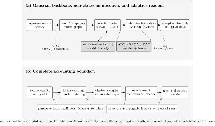
The Gaussian backbone can generate and entangle many optical or microwave modes deterministically. Universality enters through a non-Gaussian factory and adaptive measurements. A platform claim must carry source quality, loss, mode matching, detector efficiency, feedforward latency, accepted-run rate, and logical decoding through the entire boundary.

The Gaussian Backbone

A Gaussian unitary acts affinely on quadratures:

$$\mathbf R \longmapsto S\mathbf R+\mathbf s, \qquad S\Omega S^{\mathsf T} = \Omega.$$

The symplectic matrix $S$ describes phase rotations, squeezing, beam splitters, and multimode interferometers; $\mathbf s$ describes displacements. Means and covariances transform as

$$\begin{aligned} \mathbf d &\longmapsto S\mathbf d+\mathbf s, \\ V &\longmapsto SVS^{\mathsf T}. \end{aligned}$$

This compact representation is one reason Gaussian systems scale well at the control and verification layers. It is also the basis of efficient classical simulation for broad Gaussian-only circuits.

Native operations and their hardware

Primitive	Ideal action	Representative hardware	Typical imperfections
displacement	$D(\alpha)$ translates phase space	weak coherent injection, directional coupler, electro-optic drive	gain error, phase drift, finite bandwidth
phase rotation	$a\mapsto e^{-i\phi}a$	phase shifter, propagation, detuning	phase noise, dispersion, calibration drift
single-mode squeezing	$q\mapsto e^{-r}q$, $p\mapsto e^r p$	optical parametric oscillator, microring, JPA, JTWPA	loss, pump noise, excess anti-squeezing
beam splitter	mixes two modes unitarily	directional coupler, free-space or fibre coupler, microwave hybrid	imbalance, mode mismatch, insertion loss
two-mode squeezing	correlated pair creation	parametric down-conversion, four-wave mixing, Josephson mixer	thermal population, spectral impurity, pump leakage
homodyne measurement	measures $q_\theta$	local oscillator, balanced detector or IQ chain	inefficiency, electronic noise, LO phase error
feedforward	conditional displacement or basis change	FPGA, ADC/DAC, modulator, microwave drive	latency, quantization, clipping, drift

Optical devices often provide low thermal occupation and room-temperature propagation. Microwave devices provide strong, tunable Josephson nonlinearities and direct compatibility with superconducting circuits, but they require cryogenic operation and quantum-limited amplification. These are different engineering trades, not merely different carrier frequencies.

Squeezing is a source metric, not a platform verdict

An ideal squeezed vacuum has

$$V_{\rm s} = \frac{1}{2}e^{-2r}, \qquad V_{\rm a} = \frac{1}{2}e^{2r}.$$

Noise suppression is often quoted as a positive number

$$\mathcal S_{\rm dB} = -10\log_{10} \left( \frac{V_{\rm s}}{V_{\rm vac}} \right).$$

A useful report includes both squeezing and anti-squeezing, because loss, phase jitter, pump noise, and impurity affect them differently. It also includes the analysis frequency, bandwidth, optical or microwave reference plane, detection correction, uncertainty, and duration of stable operation. An inferred source value corrected for detector loss is not the same as the variance delivered to the next module.

Why Non-Gaussian Resources Are Necessary

Gaussian input states processed by Gaussian channels and measured with Gaussian detectors admit efficient phase-space descriptions. They support teleportation, dense coding, sensing, entanglement distribution, and many other nonclassical protocols, but they do not by themselves supply universal quantum computation.

One formal route to universality adds a Hamiltonian of degree greater than two in $q$ and $p$. A canonical example is the cubic phase gate

$$U_{\rm cubic}(\gamma) = \exp \left( i\gamma q^3 \right).$$

In optical hardware, a strong deterministic cubic interaction is difficult. Architectures instead prepare a non-Gaussian ancilla probabilistically and teleport its action into the data using Gaussian coupling, measurement, and feedforward. Other routes use photon subtraction or addition, photon-number resolving detection, cat-like states, or finite-energy Gottesman–Kitaev–Preskill states.

The resource can enter in three different places:

• state: a Wigner-negative or otherwise non-Gaussian ancilla is injected;
• operation: a nonlinear interaction acts directly on the data;
• measurement: photon counting or another non-Gaussian POVM conditions the output.

These routes are operationally distinct. For example, Gaussian boson sampling begins with squeezed Gaussian states and a passive Gaussian interferometer, but photon-number resolving detection is non-Gaussian. The resulting sampling problem can be classically difficult without furnishing a programmable universal gate set.

Wigner negativity is a useful resource witness, but it is not an architecture-level success criterion. The relevant quantities include prepared-state fidelity under an explicit target model, heralding probability, multiplexing overhead, loss after heralding, mode purity, repeatability, and the error of the gate or recovery operation that consumes the state.

Four Workload Classes That Must Not Be Confused

The same laboratory can support several computational models.

Workload	Information carrier	Essential resource	Appropriate output claim
Gaussian protocol	quadrature means and covariances	squeezing, Gaussian entanglement, homodyne	teleportation, communication, estimation, or sensing performance
continuous-variable measurement-based computation	quadratures on a cluster graph	finite-squeezed cluster plus adaptive measurements; non-Gaussian resource for universality	implemented channels or gates with feedforward
Gaussian boson sampling	photon-count pattern from a Gaussian state	squeezed inputs, interferometer, photon-number detection	sampling performance against specified classical methods
encoded logical computation	finite logical system inside each mode	grid, cat, or other code plus recovery and logical gates	logical error, threshold scaling, accepted resource cost

Mode count is meaningful only inside one row of this table. Thirty thousand entangled temporal modes, 216 modes in a sampling instance, and one high-quality encoded grid qubit answer different questions.

Optical Continuous-Variable Hardware

Sources and interferometers

Optical squeezing is commonly produced below threshold in an optical parametric oscillator or in a travelling-wave nonlinear medium. Second-order down-conversion and third-order four-wave mixing create correlated photon pairs, which become single- or two-mode squeezed states in an appropriate mode basis. Integrated microrings and waveguides can place source, interferometer, filtering, and phase control on a chip; bulk or fibre systems can offer lower loss or easier access during development.

The source must be characterized in the mode accepted by the processor. Spectral entanglement between an intended pulse and unobserved modes appears as mixedness. Filtering can improve purity while reducing brightness and adding loss. Pump depletion, thermal drift, parasitic nonlinear processes, and Raman or fluorescence backgrounds can make a nominally Gaussian source depart from its calibration model.

A passive $m$-mode interferometer implements

$$\mathbf a_{\rm out} = U\mathbf a_{\rm in}, \qquad U^\dagger U = I_m.$$

The matrix $U$ may be realized spatially by a mesh of beam splitters and phase shifters, temporally by recirculating delay loops, or spectrally by electro-optic modulation and pulse shaping. The abstract unitary does not show insertion loss, switching loss, finite extinction, phase-lock channels, or the number of times a pulse traverses a lossy component. Those belong in the physical transfer matrix.

Time-domain multiplexing

Time-domain multiplexing reuses one or a few squeezers, beam splitters, and detectors across a pulse train. If the clock period is $\tau$, a delay of $k\tau$ couples bins separated by $k$ steps. Several delays generate a graph with long-range edges while keeping the number of physical components nearly fixed.

This economy transfers complexity into:

• optical delay length and propagation loss;
• fast switching and phase modulation;
• clock and local-oscillator synchronization;
• accumulation of phase error over many traversals;
• detector recovery and demultiplexing;
• real-time feedforward before the target pulse leaves its delay.

Temporal depth is not automatically circuit depth. A cluster resource may contain a long stream of entangled modes while the demonstrated measurement pattern acts on only a subset or uses fixed bases.

Frequency-domain multiplexing

An optical frequency comb supplies many spectral modes from one resonator. Pump frequencies determine which mode pairs interact, and shaped polychromatic local oscillators select supermodes at readout. This can create dense or reconfigurable graphs without long spatial interferometers.

The relevant independence test is not line count alone. One should report the measured covariance matrix, mode-selectivity matrix, pump-induced cross-talk, dispersion, resonator escape efficiency, and whether the same measurement apparatus can address arbitrary graph nodes. In 2025, an integrated silicon-nitride microcomb generated and verified eight-mode continuous-variable multipartite entanglement. This established a chip-scale Gaussian entanglement module, not a universal integrated processor.

Cluster States and Measurement-Based Processing

For a graph with weighted adjacency matrix $A$, ideal cluster-state nullifiers are

$$\delta_j = p_j-\sum_k A_{jk}q_k.$$

An infinitely squeezed ideal cluster state would satisfy $\delta_j\lvert\psi_A\rangle=0$. Physical states have finite nullifier variance. Nullifier squeezing below the chosen shot-noise reference and multipartite inseparability criteria can verify a Gaussian entanglement resource.

Finite squeezing appears as additive noise during measurement-based gate teleportation. Increasing the number of modes does not reduce that noise. Fault tolerance requires a compatible encoding and recovery strategy, commonly involving finite-energy grid states and analog syndrome information, as well as loss and non-Gaussian error models beyond an ideal independent displacement channel.

Two independent 2019 experiments generated deterministic time-multiplexed two-dimensional optical cluster states. One reported more than 30,000 entangled modes in a cylindrical lattice. These were major scaling results for Gaussian resource generation. They did not include all of the non-Gaussian ancillas, adaptive logical measurements, decoders, and loss-tolerant interfaces required for universal fault-tolerant computation.

Adaptive measurement and delay

Measurement-based processing chooses a later homodyne angle or displacement from earlier outcomes. If the total electronic latency is $\tau_{\rm ff}$, the unmeasured optical pulse needs delay

$$L \geq v_g\tau_{\rm ff} = \frac{c}{n_g}\tau_{\rm ff},$$

before the conditional operation. Longer delay buys processing time at the cost of propagation loss and phase drift. The latency budget includes photodetection, analog filtering, conversion, digital computation, conversion back to analog, modulator response, and timing margin.

In 2023, nonlinear electro-optic feedforward was used to measure a nonlinear quadrature of the form

$$p+\gamma q^2.$$

With a non-Gaussian ancilla, the experiment reduced measurement excess noise by about $10\%$ relative to a vacuum ancilla. This demonstrated an important adaptive non-Gaussian measurement primitive. It did not by itself demonstrate a universal circuit or a fault-tolerant logical operation.

Microwave Continuous-Variable Hardware

Microwave continuous-variable systems use propagating or resonant modes in superconducting circuits. Josephson parametric amplifiers, Josephson parametric converters, and Josephson travelling-wave parametric amplifiers provide strong three- or four-wave mixing. Hybrid rings, circulators, directional couplers, transmission lines, and digital IQ chains implement mode mixing and measurement.

Thermal occupation

At frequency $\omega$ and temperature $T$, equilibrium thermal occupation is

$$\bar n_{\rm th} = \frac{1} {\exp\!\left(\hbar\omega/k_{\rm B}T\right)-1}.$$

Optical modes have negligible $\bar n_{\rm th}$ at room temperature. Microwave modes near a few gigahertz require millikelvin environments, cold attenuation, filtering, and careful isolation from warmer amplifier stages. The refrigerator base temperature alone does not determine the mode temperature; cable loss, pump leakage, imperfect thermalization, and backaction can raise it.

Parametric sources and frequency graphs

A pumped Josephson element can implement the two-mode-squeezing interaction

$$H_{\rm TMS} = i\hbar \left( g a_j^\dagger a_k^\dagger -g^*a_ja_k \right).$$

Multiple pump tones select multiple frequency pairs and therefore program an interaction graph. This provides a compact route to microwave frequency combs and cluster-like states, but pump crowding introduces intermodulation, gain competition, harmonics, and calibration complexity.

Milestones include two-mode microwave squeezing in 2011, deterministic remote preparation of a squeezed microwave state over $35\ {\rm cm}$ in 2019, multipartite correlations across a 64-mode Josephson parametric system in 2023, and square-ladder microwave cluster states in 2025. A 2026 Josephson travelling-wave experiment programmed four-mode linear, cyclic, star, and fully connected graphs by changing pump tones. Its reported nullifier squeezing was below $1\ {\rm dB}$ for those graphs, and the authors explicitly identified much larger states, substantially stronger squeezing, and a non-Gaussian resource as requirements for fault-tolerant computation.

These results establish increasingly flexible Gaussian microwave networks. They should not be described as complete microwave continuous-variable computers.

Amplifier noise and calibration

Phase-preserving amplification necessarily adds noise. Reconstructing an input covariance from room-temperature IQ records therefore requires a calibrated gain and noise model. Pump-on/pump-off subtraction can remove the mean contribution of a stable readout chain, but it does not automatically remove drift, compression, correlated amplifier noise, or uncertainty in the reference state.

Useful reports separate:

• squeezing generated at the device;
• squeezing delivered after cryogenic loss;
• noise observed at the digitizer;
• values inferred after readout-chain correction.

That separation is as important for microwaves as separating on-chip and off-chip loss is for optics.

Initialization, Gates, and Readout

Initialization

Gaussian initialization can be deterministic: cool or evacuate the mode, displace it, squeeze it, and entangle it with other modes. Non-Gaussian initialization is usually more costly. Photon detection may herald a conditioned optical state; a superconducting ancilla may synthesize a cavity state; breeding or distillation may combine several imperfect resources.

For a heralded resource with per-attempt probability $p_{\rm h}$, multiplexing $N$ independent attempts gives

$$p_{\geq 1} = 1-(1-p_{\rm h})^N.$$

This improves availability only if successful states can be routed into the processor with sufficiently low loss and latency. Switches, buffers, and discarded attempts are part of the cost.

Gates

Gaussian gates can be direct interferometric transformations or measurement-induced operations. A non-Gaussian gate can be teleported from an ancilla, conditioned on a detector result, or mediated by a nonlinear matter degree of freedom. The reported gate error should include ancilla quality, coupling loss, detector error, feedforward, and any acceptance rule.

An operation demonstrated on coherent or squeezed probes need not have the same fidelity on a Wigner-negative input. Process characterization should cover the energy and phase-space region used by the algorithm or logical code.

Homodyne, heterodyne, and photon counting

Homodyne detection measures one quadrature selected by a local-oscillator phase. It can be efficient and fast, but phase error rotates anti-squeezed noise into the measured quadrature. Heterodyne detection obtains both quadratures at the cost of an additional vacuum contribution in the ideal model.

Photon-number resolving detection supplies a non-Gaussian measurement. Its relevant metrics are system efficiency, number resolution, dark counts, timing jitter, saturation, reset time, and maximum sustainable event rate. A detector with excellent intrinsic efficiency can still sit behind lossy coupling, filtering, switching, and interferometry.

Noise and Error Ledger

Loss

A thermal-loss channel with power transmissivity $\eta$ maps covariance as

$$V_{\rm out} = \eta V_{\rm in} + (1-\eta) \frac{2\bar n_{\rm env}+1}{2}I.$$

For a squeezed quadrature,

$$V_{{\rm s,out}} = \frac{1}{2} \left[ \eta e^{-2r} + (1-\eta)(2\bar n_{\rm env}+1) \right].$$

At optical frequencies the environment is usually well approximated by vacuum, but loss still replaces the state with vacuum and destroys non-Gaussian features. At microwave frequencies, a warm environment can add thermal photons as well.

If independent components have efficiencies $\eta_1,\ldots,\eta_n$, then

$$\eta_{\rm tot} = \prod_{j=1}^{n}\eta_j.$$

Small losses therefore compound rapidly in looped or deeply multiplexed architectures.

Phase noise

If the intended squeezed axis is measured with angular error $\delta\theta$, the observed variance is

$$V(\delta\theta) = V_{\rm s}\cos^2\delta\theta + V_{\rm a}\sin^2\delta\theta.$$

Strong squeezing brings strong anti-squeezing, so improving the source can increase sensitivity to phase jitter. Quoting only the best squeezed variance hides this systems trade.

Mode mismatch and leakage

Imperfect overlap at a beam splitter acts partly like loss and partly like coupling to an unwanted distinguishable mode. In a multiplexed processor, spectral or temporal leakage can also create correlated errors between bins. The mode-overlap matrix should be measured under the same switching and pump conditions used for computation.

Finite squeezing

Finite squeezing adds noise to cluster-state teleportation and broadens finite-energy grid-state peaks. It is not a small implementation detail that can be removed by declaring more modes. Error-correction thresholds depend on the full distribution of shifts, loss events, envelope distortion, and measurement error, not on a single squeezing number.

Pump and electronics noise

Parametric gain depends on pump amplitude and phase. Pump fluctuations, spurious sidebands, harmonics, and leakage into detectors can create correlated nonstationary noise. ADC resolution, DAC update rate, analog bandwidth, clipping, and FPGA arithmetic determine whether a feedforward law is implemented over the required dynamic range.

Resource-state yield

If a useful output requires source success, transmission, switching, detection, and acceptance, a schematic rate is

$$R_{\rm acc} = R_{\rm clock} p_{\rm source} \eta_{\rm path} \eta_{\rm det} p_{\rm accept}.$$

For several required heralds these factors may enter with powers or more complicated multiplexing statistics. Reporting only $R_{\rm clock}$ can overstate useful throughput by orders of magnitude.

Connectivity and Scaling

Continuous-variable platforms can expose large mode graphs because modes are cheap to generate and interfere. The graph can live in:

• spatial paths and interferometer meshes;
• temporal bins and recirculating delays;
• frequency bins and pump-selected couplings;
• polarization or orbital modes;
• hybrid combinations of these degrees of freedom.

For architecture comparison, specify at least four graphs:

1. the state graph inferred from covariance or higher moments;
2. the control graph of independently programmable transformations;
3. the measurement graph of adaptively addressable modes;
4. the logical graph after encoding, recovery, and accepted failures.

These graphs need not coincide. A source can generate a dense covariance graph while the controller addresses only global supermodes. A loop can create long-range temporal edges while loss limits usable depth. A logical grid-state architecture can consume many physical modes per surviving logical node.

Scaling claims should therefore report mode number together with squeezing, loss per layer or loop, graph degree, programmable parameters, adaptive depth, calibration time, non-Gaussian resource rate, and output metric.

Metrics for Fair Comparison

Source and Gaussian-state metrics

Report:

• squeezed and anti-squeezed variances at a named reference plane;
• state purity or symplectic eigenvalues;
• bandwidth and mode count with explicit mode definitions;
• phase stability and drift over operational time;
• covariance uncertainty and physicality checks;
• entanglement witnesses with their assumptions.

For a measured covariance matrix, the uncertainty principle requires

$$V+\frac{i}{2}\Omega \geq 0.$$

A reconstructed matrix that violates this condition beyond uncertainty usually signals calibration or estimation problems, not a more quantum state.

Cluster metrics

Nullifier variances should be normalized to a clearly defined shot-noise reference and accompanied by a multipartite inseparability test where appropriate. Graph size alone is insufficient. Report whether the graph was generated, verified, reconfigured, measured adaptively, and consumed in a gate sequence.

Non-Gaussian metrics

Report:

• Wigner negativity or another resource witness with uncertainty;
• target-state fidelity under a stated finite-energy model;
• heralding probability and accepted rate;
• photon-number resolution and total efficiency;
• resource degradation after switching and storage;
• the error of the operation that consumes the resource.

Computational and logical metrics

A sampling claim needs a specified distribution, validation tests, classical competitors, runtime boundary, and postselection policy. A fault-tolerance claim needs logical error versus code size or resource quality, including non-Gaussian preparation, recovery, feedforward, and discarded runs.

Metrics for Quantum Hardware develops uncertainty-aware fidelity and benchmarking principles. The continuous-variable addition is that mode quality, energy, covariance conventions, and acceptance probabilities must remain visible.

Evidence Through August 2026

The following milestones support different layers of the architecture.

Year	Result	What it established	What remained open
1998	unconditional optical continuous-variable teleportation	deterministic Gaussian entanglement, Bell measurement, and feedforward	scalable computation and fault tolerance
2013	time-multiplexed cluster state with 10,000 modes	extreme Gaussian temporal multiplexing	two-dimensional fault-tolerant resource and non-Gaussian layer
2019	deterministic two-dimensional optical cluster states	large two-dimensional Gaussian resource graphs; one exceeded 30,000 modes	universal adaptive logical processing
2022	216-mode programmable Borealis experiment	time-multiplexed Gaussian boson sampling with photon-number detection and a computational-advantage claim	universal gates, error correction, useful logical computation
2023	nonlinear optical feedforward	fast adaptive nonlinear quadrature measurement with a non-Gaussian ancilla	integration with a full logical processor
2023–2026	increasingly structured microwave frequency graphs	multipartite Gaussian microwave entanglement and pump-programmable cluster graphs	stronger squeezing, much larger graphs, non-Gaussian resources, adaptive logical operations
2025	eight-mode integrated optical microcomb entanglement	chip-scale deterministic multimode Gaussian source and programmable measurement basis	integrated universal processor
2025	integrated optical grid-state source	resolved grid structure and Wigner negativity in both quadratures	lower loss, higher effective squeezing, array yield, recovery, logical gates
2026	unified optical non-Gaussian resource proposal	a peer-reviewed numerical and architectural framework using Gaussian inputs, amplification, and heralded detection	experimental realization and end-to-end loss/yield validation

The Borealis experiment used 216 squeezed modes, a programmable time-multiplexed interferometer, and photon-number resolving detectors, with up to 219 detected photons in reported samples. It was a sophisticated Gaussian boson sampler. Its non-Gaussian measurement and sampling evidence should not be translated into a claim of universal continuous-variable computation.

The 2025 integrated optical grid-state experiment showed four resolvable peaks in each quadrature and a $3\times3$ pattern of Wigner-negative regions. The authors explicitly described further optical-loss reduction as necessary for fault-tolerant use. It is best classified as a source milestone.

The July 2026 unified optical framework reports numerical state-generation fidelities and a route to breeding finite-energy grid states using Gaussian inputs, optical parametric amplification, and heralded detection. It is a published architecture and modelling result, not an experimental fault-tolerant processor.

As of 10 August 2026, no optical or microwave platform has demonstrated a complete universal fault-tolerant continuous-variable processor with end-to-end logical error suppression and full resource accounting.

Advantages and Bottlenecks

Structural advantages

• Gaussian entangling operations and homodyne measurements can be deterministic.
• Temporal and frequency multiplexing can create very large mode graphs with few repeated components.
• Optical modes propagate at room temperature and interface naturally with communication networks.
• Microwave modes couple strongly to superconducting circuits and can use programmable Josephson nonlinearities.
• Analog measurement outcomes can provide soft information to decoders.
• The same hardware supports computation, communication, and sensing primitives.

Central bottlenecks

• optical loss rapidly erases squeezing and non-Gaussianity;
• finite squeezing becomes gate noise rather than disappearing at large mode count;
• deterministic strong non-Gaussian interactions are difficult;
• heralded resources require routing, buffering, and high total efficiency;
• adaptive processing ties electronics latency to physical delay and loss;
• mode selectivity, phase locking, and calibration become harder at scale;
• microwave platforms must control thermal photons and amplifier noise;
• logical thresholds depend on realistic correlated and non-Gaussian errors;
• accepted logical throughput can be far below the source clock.

The attractive Gaussian backbone and the difficult non-Gaussian frontier are both real. Trustworthy evaluation keeps them in the same accounting model.

Claim Audit

Before accepting a continuous-variable hardware claim, ask:

1. What is the exact mode basis, and how was orthogonality verified?
2. Which reference plane defines the quoted squeezing and efficiency?
3. Are both squeezing and anti-squeezing reported?
4. Was the full covariance matrix physical within uncertainty?
5. What operation or measurement supplies non-Gaussianity?
6. Is the non-Gaussian result measured, inferred, simulated, or proposed?
7. What is the heralding and accepted-run rate?
8. How much loss occurs after resource preparation?
9. Was the graph merely generated, or also reconfigured and measured adaptively?
10. Does a computational claim concern Gaussian protocols, sampling, universal gates, or encoded logical computation?
11. Which classical simulation and spoofing methods were tested?
12. Does logical error improve with code size or resource quality under a complete noise model?

Common Mistakes

Equating many modes with many logical qubits

A mode is an infinite-dimensional carrier, not automatically a protected logical qubit. Cluster nodes, sampling modes, and grid-encoded logical qubits have different resource meanings.

Calling every squeezed-light experiment universal

Squeezing is a Gaussian resource. Universal computation requires a non-Gaussian state, operation, or measurement integrated into the processing model.

Treating loss-corrected squeezing as delivered squeezing

Correcting detector inefficiency can estimate source performance, but the next module receives the uncorrected state. Both values should be reported.

Ignoring anti-squeezing

Phase jitter mixes anti-squeezed noise into the protected quadrature. Squeezing without anti-squeezing and phase stability is incomplete.

Calling a hard sampler a universal computer

Classical hardness of a sampling distribution does not imply a programmable universal gate set or fault-tolerant logical operations.

Calling a source a processor

A high-quality non-Gaussian or grid-state source can solve a crucial bottleneck while leaving routing, fusion, recovery, feedforward, and logical benchmarking undone.

Counting clock rate instead of accepted output rate

Heralding, switching, transmission, detector efficiency, and acceptance can reduce useful throughput far below the pulse or pump rate.

Exercises

1. Verify the quadrature convention

Starting from $[a,a^\dagger]=1$, verify $[q,p]=i$ for the quadratures used on this page. Show that the vacuum variances are $1/2$.

Solution

The commutator is

$$\begin{aligned} [q,p] &= \frac{1}{i2} [a+a^\dagger,a-a^\dagger] \\ &= \frac{1}{i2} \left( -[a,a^\dagger] +[a^\dagger,a] \right) \\ &= i. \end{aligned}$$

Since $a\lvert0\rangle=0$ and $\langle0\rvert aa^\dagger\lvert0\rangle=1$,

$$\langle q^2\rangle_0 = \langle p^2\rangle_0 = \frac{1}{2},$$

while both means vanish.

2. Send squeezed light through loss

An optical source produces $10\ {\rm dB}$ of ideal squeezing and then passes through a vacuum-loss channel with $\eta=0.80$. What squeezing is observed?

Solution

Ten decibels means

$$\frac{V_{\rm s}}{V_{\rm vac}} = 10^{-10/10} = 0.1.$$

Vacuum loss gives

$$\frac{V_{{\rm s,out}}}{V_{\rm vac}} = \eta(0.1)+(1-\eta) = 0.28.$$

Therefore

$$\mathcal S_{\rm out} = -10\log_{10}(0.28) \approx 5.53\ {\rm dB}.$$

A $20\%$ loss removes almost half of the quoted noise suppression in decibel terms.

3. Quantify phase-jitter contamination

A state has $V_{\rm s}=0.05$ and $V_{\rm a}=5.0$ in units where vacuum variance is $0.5$. Find the observed variance for a fixed phase error of $2^\circ$. Compare it with the ideal squeezed variance.

Solution

Using $\delta\theta=2\pi/180$,

$$\begin{aligned} V(\delta\theta) &= 0.05\cos^2\delta\theta + 5.0\sin^2\delta\theta \\ &\approx 0.0560. \end{aligned}$$

The variance increases by about $12\%$. The absolute angle is small, but the large anti-squeezed variance amplifies its effect.

4. Compare microwave thermal occupations

Estimate $\bar n_{\rm th}$ for a $5\ {\rm GHz}$ mode at $20\ {\rm mK}$ and $100\ {\rm mK}$. Use $h f/k_{\rm B}\approx0.240\ {\rm K}$.

Solution

At fixed frequency,

$$\bar n_{\rm th} = \frac{1}{e^{hf/(k_{\rm B}T)}-1}.$$

At $20\ {\rm mK}$,

$$\bar n_{\rm th} \approx \frac{1}{e^{12}-1} \approx 6.1\times10^{-6}.$$

At $100\ {\rm mK}$,

$$\bar n_{\rm th} \approx \frac{1}{e^{2.4}-1} \approx 0.10.$$

The fivefold temperature increase changes the mode from nearly vacuum to roughly one thermal photon per ten modes on average.

5. Check a beam splitter

For

$$\begin{pmatrix} a_1'\\ a_2' \end{pmatrix} = \begin{pmatrix} \sqrt{\eta}&\sqrt{1-\eta}\\ -\sqrt{1-\eta}&\sqrt{\eta} \end{pmatrix} \begin{pmatrix} a_1\\ a_2 \end{pmatrix},$$

verify that $[a_j',a_k'^\dagger]=\delta_{jk}$.

Solution

The mixing matrix $U$ is real and satisfies

$$UU^\dagger = \begin{pmatrix} \eta+1-\eta&0\\ 0&1-\eta+\eta \end{pmatrix} = I.$$

Therefore

$$\begin{aligned} [a_j',a_k'^\dagger] &= \sum_{\ell,m} U_{j\ell}U_{km}^* [a_\ell,a_m^\dagger] \\ &= (UU^\dagger)_{jk} \\ &= \delta_{jk}. \end{aligned}$$

The minus sign is needed to make the two rows orthogonal.

6. Size an optical feedforward delay

An adaptive controller has total latency $64\ {\rm ns}$. Estimate the minimum fibre length for group index $n_g=1.5$. Why will a laboratory delay usually be longer?

Solution

The group velocity is $c/n_g$, so

$$\begin{aligned} L_{\min} &= \frac{c\tau_{\rm ff}}{n_g} \\ &= \frac{ (3.00\times10^8) (64\times10^{-9}) }{1.5} \ {\rm m} \\ &\approx 12.8\ {\rm m}. \end{aligned}$$

A real setup needs timing margin, connector and component delays, pulse separation, and enough fibre to place modulators and detectors conveniently. The added length also adds loss and phase sensitivity.

7. Compound an efficiency budget

A heralded state passes through coupling with efficiency $0.95$, three loop traversals each with efficiency $0.97$, a switch with efficiency $0.94$, and a detector with efficiency $0.98$. Find the end-to-end efficiency.

Solution

The efficiencies multiply:

$$\begin{aligned} \eta_{\rm tot} &= 0.95 (0.97)^3 (0.94) (0.98) \\ &\approx 0.798. \end{aligned}$$

Thus about $20\%$ of events are lost even though every individual component exceeds $94\%$ efficiency.

8. Interpret a cluster nullifier

For a three-node line with unit-weight edges, write the three nullifiers. What does a measured nonzero variance mean?

Solution

With edges $1$–$2$ and $2$–$3$,

$$\begin{aligned} \delta_1 &= p_1-q_2, \\ \delta_2 &= p_2-q_1-q_3, \\ \delta_3 &= p_3-q_2. \end{aligned}$$

An ideal infinitely squeezed cluster state would have zero variance for every nullifier. A physical nonzero variance reflects finite squeezing plus loss, phase error, mode mismatch, and detector noise. Variance below a stated shot-noise bound can witness the intended correlations, but it does not by itself demonstrate universal computation.

9. Compute accepted resource throughput

A source is clocked at $10\ {\rm MHz}$. It heralds a usable ancilla with probability $0.02$, the path efficiency is $0.75$, detector efficiency is $0.95$, and $80\%$ of detected events pass a quality cut. Estimate the accepted rate.

Solution

The schematic rate is

$$\begin{aligned} p_{\rm tot} &= (0.02)(0.75)(0.95)(0.80) \\ &= 0.0114, \\ R_{\rm acc} &= (10^7\ {\rm s^{-1}})p_{\rm tot} \\ &= 1.14\times10^5\ {\rm s^{-1}}. \end{aligned}$$

The useful rate is $114\ {\rm kHz}$, not the $10\ {\rm MHz}$ source clock. If several independent ancillas are needed simultaneously, the rate can fall much more sharply unless multiplexing is included.

10. Classify hardware claims

Assign the strongest justified claim to each result:

1. a 30,000-mode Gaussian cluster resource with fixed measurements;
2. a 216-mode squeezed-state interferometer sampled by photon-number detectors;
3. an integrated source with grid peaks and Wigner negativity;
4. decreasing logical error with increasing code size during universal operations.

Solution

1. Large-scale Gaussian entanglement generation. It establishes multiplexed resource-state scaling, not universal logical processing.
2. Programmable Gaussian boson sampling. The photon-counting measurement is non-Gaussian and may support a computational-hardness result, but the device is not thereby a universal gate processor.
3. Non-Gaussian encoded-state source milestone. It establishes important state structure; loss, source arrays, recovery, gates, and logical scaling remain.
4. Fault-tolerant logical evidence, provided the comparison uses matched tasks, complete acceptance accounting, and all preparation, recovery, and measurement faults. This is the architecture-level target not yet reached by continuous-variable hardware.

References

1. S. L. Braunstein and P. van Loock, “Quantum Information with Continuous Variables,” Reviews of Modern Physics 77, 513–577 (2005), doi:10.1103/RevModPhys.77.513.
2. C. Weedbrook et al., “Gaussian Quantum Information,” Reviews of Modern Physics 84, 621–669 (2012), doi:10.1103/RevModPhys.84.621.
3. S. Lloyd and S. L. Braunstein, “Quantum Computation over Continuous Variables,” Physical Review Letters 82, 1784–1787 (1999), doi:10.1103/PhysRevLett.82.1784.
4. S. D. Bartlett, B. C. Sanders, S. L. Braunstein, and K. Nemoto, “Efficient Classical Simulation of Continuous Variable Quantum Information Processes,” Physical Review Letters 88, 097904 (2002), doi:10.1103/PhysRevLett.88.097904.
5. A. Mari and J. Eisert, “Positive Wigner Functions Render Classical Simulation of Quantum Computation Efficient,” Physical Review Letters 109, 230503 (2012), doi:10.1103/PhysRevLett.109.230503.
6. N. C. Menicucci et al., “Universal Quantum Computation with Continuous-Variable Cluster States,” Physical Review Letters 97, 110501 (2006), doi:10.1103/PhysRevLett.97.110501.
7. M. Gu, C. Weedbrook, N. C. Menicucci, T. C. Ralph, and P. van Loock, “Quantum Computing with Continuous-Variable Clusters,” Physical Review A 79, 062318 (2009), doi:10.1103/PhysRevA.79.062318.
8. N. C. Menicucci, “Fault-Tolerant Measurement-Based Quantum Computing with Continuous-Variable Cluster States,” Physical Review Letters 112, 120504 (2014), doi:10.1103/PhysRevLett.112.120504.
9. D. Gottesman, A. Kitaev, and J. Preskill, “Encoding a Qubit in an Oscillator,” Physical Review A 64, 012310 (2001), doi:10.1103/PhysRevA.64.012310.
10. K. Fukui, A. Tomita, A. Okamoto, and K. Fujii, “High-Threshold Fault-Tolerant Quantum Computation with Analog Quantum Error Correction,” Physical Review X 8, 021054 (2018), doi:10.1103/PhysRevX.8.021054.
11. A. Furusawa et al., “Unconditional Quantum Teleportation,” Science 282, 706–709 (1998), doi:10.1126/science.282.5389.706.
12. S. Yokoyama et al., “Ultra-Large-Scale Continuous-Variable Cluster States Multiplexed in the Time Domain,” Nature Photonics 7, 982–986 (2013), doi:10.1038/nphoton.2013.287.
13. W. Asavanant et al., “Generation of Time-Domain-Multiplexed Two-Dimensional Cluster State,” Science 366, 373–376 (2019), doi:10.1126/science.aay2645.
14. M. V. Larsen, X. Guo, C. R. Breum, J. S. Neergaard-Nielsen, and U. L. Andersen, “Deterministic Generation of a Two-Dimensional Cluster State,” Science 366, 369–372 (2019), doi:10.1126/science.aay4354.
15. L. S. Madsen et al., “Quantum Computational Advantage with a Programmable Photonic Processor,” Nature 606, 75–81 (2022), doi:10.1038/s41586-022-04725-x.
16. A. Sakaguchi et al., “Nonlinear Feedforward Enabling Quantum Computation,” Nature Communications 14, 3817 (2023), doi:10.1038/s41467-023-39195-w.
17. H. Vahlbruch et al., “Detection of 15 dB Squeezed States of Light and Their Application for the Absolute Calibration of Photoelectric Quantum Efficiency,” Physical Review Letters 117, 110801 (2016), doi:10.1103/PhysRevLett.117.110801.
18. X. Jia et al., “Continuous-Variable Multipartite Entanglement in an Integrated Microcomb,” Nature 639, 329–336 (2025), doi:10.1038/s41586-025-08602-1.
19. M. V. Larsen et al., “Integrated Photonic Source of Gottesman–Kitaev–Preskill Qubits,” Nature (2025), doi:10.1038/s41586-025-09044-5.
20. Ö. Erkılıç et al., “A Unified Optical Platform for Non-Gaussian and Fault-Tolerant Gottesman–Kitaev–Preskill States,” npj Quantum Information (2026), doi:10.1038/s41534-026-01336-6.
21. X. Su et al., “Gate Sequence for Continuous Variable One-Way Quantum Computation,” Nature Communications 4, 2828 (2013), doi:10.1038/ncomms3828.
22. N. C. Menicucci, “Temporal-Mode Continuous-Variable Cluster States Using Linear Optics,” Physical Review A 83, 062314 (2011), doi:10.1103/PhysRevA.83.062314.
23. C. Eichler et al., “Observation of Two-Mode Squeezing in the Microwave Frequency Domain,” Physical Review Letters 107, 113601 (2011), doi:10.1103/PhysRevLett.107.113601.
24. E. Flurin, N. Roch, F. Mallet, M. H. Devoret, and B. Huard, “Generating Entangled Microwave Radiation over Two Transmission Lines,” Physical Review Letters 109, 183901 (2012), doi:10.1103/PhysRevLett.109.183901.
25. S. Pogorzalek et al., “Secure Quantum Remote State Preparation of Squeezed Microwave States,” Nature Communications 10, 2604 (2019), doi:10.1038/s41467-019-10727-7.
26. K. V. Petrovnin et al., “Generation and Structuring of Multipartite Entanglement in a Josephson Parametric System,” Physical Review Letters 130, 120601 (2023), doi:10.1103/PhysRevLett.130.120601.
27. F. Lingua, J. C. Rivera Hernández, M. Cortinovis, and D. B. Haviland, “Continuous-Variable Square-Ladder Cluster States in a Microwave Frequency Comb,” Physical Review Letters 134, 183602 (2025), doi:10.1103/PhysRevLett.134.183602.
28. A. Alocco et al., “Programmable Microwave Cluster States via Josephson Metamaterials,” Nature Communications (2026), doi:10.1038/s41467-026-74377-2.
29. C. M. Caves, “Quantum Limits on Noise in Linear Amplifiers,” Physical Review D 26, 1817–1839 (1982), doi:10.1103/PhysRevD.26.1817.
30. P. van Loock and A. Furusawa, “Detecting Genuine Multipartite Continuous-Variable Entanglement,” Physical Review A 67, 052315 (2003), doi:10.1103/PhysRevA.67.052315.
31. K. Marshall, R. Pooser, G. Siopsis, and C. Weedbrook, “Repeat-Until-Success Cubic Phase Gate for Universal Continuous-Variable Quantum Computation,” Physical Review A 91, 032321 (2015), doi:10.1103/PhysRevA.91.032321.
32. M. Walschaers, “Non-Gaussian Quantum States and Where to Find Them,” PRX Quantum 2, 030204 (2021), doi:10.1103/PRXQuantum.2.030204.

Further Connections

• Hardware Overview supplies the platform-neutral architecture contract and claim ladder.
• Control, Readout, and Calibration treats feedback loops, detector assignment, drift, and controller validation across hardware families.
• Bosonic Qubits develops the finite-dimensional encoded alternative inside oscillator modes.
• Photonic Qubits develops discrete photonic encodings and source-to-detector loss accounting.
• Superconducting Qubits connects microwave modes, Josephson nonlinearities, and circuit-QED control.
• Quantum Information Roadmap places modes and Gaussian processing before hardware comparison, error correction, and logical benchmarking.