Potential Energy Surfaces

A molecular potential energy surface assigns an energy to every admissible nuclear geometry for a specified electronic state and electronic Hamiltonian. Its minima organize stable structures, its curvature controls small-amplitude vibration, its saddle regions organize candidate reaction pathways, and its asymptotes identify dissociation channels.

The word surface is historical. A nonlinear molecule with $N_N$ nuclei has $3N_N-6$ internal coordinates, so the object is usually a scalar field in a high-dimensional shape space rather than a literal two-dimensional surface. A contour plot is a projection or slice of that field.

This page owns the geometry and practical use of molecular energy landscapes:

• what object is being called a potential energy surface;
• how coordinates, metrics, and symmetry affect its representation;
• how minima, saddles, reaction paths, and barriers are defined;
• what can and cannot be inferred from a surface alone;
• how crossings require a multistate description;
• how analytic, interpolated, and machine-learned surfaces are constructed and validated.

Born–Oppenheimer in Molecules owns the molecular separation of electronic and nuclear motion. Born–Oppenheimer Approximation as Scale Separation owns the exact channel equations and error logic. H₂⁺ Ion is the canonical one-dimensional example in which the electronic eigenvalue, nuclear repulsion, dissociation zero, well depth, and nuclear potential can all be followed explicitly. This page begins after the fixed-geometry electronic problem has been posed.

Nonadiabatic Coupling owns dynamics among surfaces and the assumptions behind trajectory, wavepacket, and vibronic descriptions.

Conical Intersections owns exact degeneracy conditions, seam dimension, branching-plane geometry, MECIs, and conical-intersection diagnostics.

The Defining Eigenvalue Problem

Let $R$ denote a complete nuclear geometry after overall translation has been removed. For each fixed $R$, solve

$$H_e(R) \lvert\phi_a(R)\rangle = E_a(R) \lvert\phi_a(R)\rangle.$$

Throughout this page, $H_e(R)$ includes the internuclear repulsion. The Born–Oppenheimer surface for electronic state $a$ is therefore

$$U_a^{\mathrm{BO}}(R)=E_a(R).$$

Some authors reserve $E_a$ for the electronic energy without internuclear repulsion and write

$$U_a(R) = \mathcal E_a(R)+V_{NN}(R).$$

These conventions describe the same physics when translated consistently. A quoted minimum or barrier is ambiguous unless the electronic state, Hamiltonian, energy zero, and correction level are stated.

One geometry, several electronic states

The electronic Hamiltonian has a family of eigenvalues,

$$E_0(R),E_1(R),E_2(R),\ldots,$$

so a molecule generally has many potential energy surfaces. A label such as “the surface” usually means one specified electronic state over one specified region. Energy ordering is not always a reliable identity label: near avoided crossings, states can exchange character while their ordered eigenvalues remain smooth.

Spin, spatial symmetry, charge, and asymptotic channel labels help identify states. In computations, overlaps, transition properties, and reduced density matrices may be needed to track electronic character from one geometry to the next.

Born–Oppenheimer and adiabatic surfaces

Terminology is not completely uniform. A useful distinction is:

$$\begin{aligned} U_a^{\mathrm{BO}}(R) &=E_a(R), \\ U_a^{\mathrm{ad}}(R) &=E_a(R)+\Phi_a(R), \end{aligned}$$

where $\Phi_a$ is the diagonal Born–Oppenheimer correction, or DBOC. In a simple Cartesian representation,

$$\begin{aligned} \Phi_a(R) = \sum_A\frac{\hbar^2}{2M_A} \bigg[ &\langle\nabla_A\phi_a \vert \nabla_A\phi_a\rangle_e \\ &- \lvert \langle\phi_a \vert \nabla_A\phi_a\rangle_e \rvert^2 \bigg]. \end{aligned}$$

The projected form is gauge invariant. It also shows that the corrected surface depends on nuclear masses, whereas the clamped-nuclei Born–Oppenheimer surface does not. Relativistic, radiative, finite-nuclear-size, external-field, and environmental corrections define still other effective surfaces.

Geometry Space, Not a Coordinate List

For $N_N$ distinct nuclei away from collisions, labeled Cartesian configurations lie in

$$\begin{gathered} R=(\mathbf R_1,\ldots,\mathbf R_{N_N}), \\ \widetilde{\mathcal Q} = \{R\in\mathbb R^{3N_N}: \mathbf R_A\ne\mathbf R_B\}. \end{gathered}$$

Overall translations and rotations do not change an isolated molecule’s internal shape. Schematically, its shape space is

$$\mathcal Q = \widetilde{\mathcal Q}/SE(3),$$

with further identifications under permutations of identical nuclei. Away from singular geometries, a nonlinear molecule has

$$f=3N_N-6$$

internal degrees of freedom; a linear molecule has $f=3N_N-5$. Collinear geometries, collisions, and highly symmetric arrangements require local care because a single global coordinate chart need not exist.

Coordinate representations

Common coordinates include:

• Cartesian positions with translation and rotation projected out;
• bond lengths, bond angles, and dihedral angles;
• Jacobi coordinates for fragmentation and scattering;
• symmetry-adapted coordinates;
• mass-weighted normal coordinates near a stationary point;
• invariant distances or descriptors for fitted potentials.

The numerical function written as $U(q^1,\ldots,q^f)$ changes its appearance under a coordinate transformation, but the energy assigned to a physical geometry does not.

Gradients need a metric

The differential

$$dU = \sum_i \frac{\partial U}{\partial q^i} dq^i$$

is coordinate covariant. To convert it into a steepest-descent vector, one needs a metric $G_{ij}(q)$. If the classical nuclear kinetic energy is

$$T_N = \frac12 \sum_{ij} G_{ij}(q) \dot q^i\dot q^j,$$

then

$$\left(\operatorname{grad}_G U\right)^i = \sum_jG^{ij} \frac{\partial U}{\partial q^j}.$$

Thus “steepest descent” is incomplete without a coordinate metric. Mass-weighted Cartesian coordinates supply the metric used by the conventional intrinsic reaction coordinate.

Forces and electronic response

In Cartesian coordinates, the force on nucleus $A$ is

$$\mathbf F_A(R) = -\nabla_AU(R).$$

For an exact, normalized, nondegenerate electronic eigenstate in a fixed representation, the Hellmann–Feynman theorem gives

$$\nabla_AE_a(R) = \langle\phi_a(R) \vert \nabla_AH_e(R) \vert \phi_a(R)\rangle_e.$$

Approximate wavefunctions, incomplete optimization, and atom-centered bases can require response and Pulay terms. A smooth-looking energy fit can also have poor derivatives; forces must be validated as first-class observables of the representation.

What a Surface Is Not

A PES is indispensable, but several neighboring objects must remain distinct.

Object	Precise meaning
Born–Oppenheimer surface	A clamped-nuclei electronic eigenvalue $E_a(R)$, with a stated convention for $V_{NN}$
Corrected adiabatic surface	$E_a(R)$ plus specified diagonal finite-mass or other corrections
Diabatic model	A smooth matrix $W_{ab}(R)$ whose eigenvalues reproduce coupled adiabatic surfaces
Force field	An analytic or learned approximation $\widetilde U(R)$, often with a restricted chemical domain
Free-energy profile	A temperature- and ensemble-dependent reduction in which other coordinates have been averaged
Molecular spectrum	Eigenvalues or resonances obtained only after nuclear motion and required couplings are included

A PES is not directly observed as a complete function. Experiments constrain it through rovibrational levels, scattering cross sections, reaction rates, equilibrium structures, diffraction data, and other observables after a nuclear model has been supplied. Inverse reconstruction is therefore model dependent and may be nonunique.

Nor is a surface an exact molecular spectrum with the nuclei permanently fixed. Zero-point motion, rotation, tunneling, exchange symmetry, nonadiabatic coupling, and external conditions still matter.

Stationary Points and Molecular Structure

A stationary geometry $q_*$ satisfies

$$\begin{gathered} \left. \dfrac{\partial U}{\partial q^i} \right|_{q_*} =0, \\ i=1,\ldots,f. \end{gathered}$$

Its local character is determined by the Hessian

$$K_{ij}(q_*) = \left. \frac{\partial^2U} {\partial q^i\partial q^j} \right|_{q_*}.$$

After translations, rotations, constraints, and redundant coordinates have been handled, the index is the number of negative Hessian eigenvalues:

Index	Local interpretation
$0$	minimum
$1$	first-order saddle; candidate elementary transition structure
$2$ or higher	higher-order saddle

A positive-semidefinite Cartesian Hessian with six zero eigenvalues is not yet evidence of six floppy vibrations: for a nonlinear isolated molecule those zero modes represent three translations and three rotations. A linear molecule has five such external zero modes.

Why the classification is coordinate independent

Under a smooth nonsingular change $q=q(Q)$, the Hessian transforms as

$$\begin{aligned} \frac{\partial^2U} {\partial Q^\alpha\partial Q^\beta} = &\sum_{ij} \frac{\partial q^i}{\partial Q^\alpha} K_{ij} \frac{\partial q^j}{\partial Q^\beta} \\ &+ \sum_i \frac{\partial U}{\partial q^i} \frac{\partial^2q^i} {\partial Q^\alpha\partial Q^\beta}. \end{aligned}$$

At a stationary point, the second line vanishes. The remaining congruence transformation preserves the numbers of positive, negative, and zero directions. Away from a stationary point, an ordinary coordinate Hessian is not a tensor; covariant derivatives or a specified coordinate convention are required.

Local, global, and symmetry-related minima

A local minimum is lower than nearby geometries. A global minimum is lowest over the stated domain and electronic state. Distinct local minima may be conformers, structural isomers, or symmetry-related copies of one physical arrangement.

The lowest electronic minimum need not be the most populated structure at finite temperature. Entropy, zero-point energy, nuclear spin statistics, and barriers between basins affect observed populations and interconversion.

Equilibrium versus averaged structure

The minimum $R_e$ of an electronic surface is an equilibrium geometry in the clamped-nuclei model. A rotationally or vibrationally inferred structure samples a nuclear wavefunction and is generally different:

$$\langle R\rangle_\nu \ne R_e.$$

Isotope substitution leaves $U^{\mathrm{BO}}(R)$ unchanged to leading order but changes the nuclear wavefunction, vibrational averaging, zero-point energy, and the DBOC. This distinction matters in precision structural work.

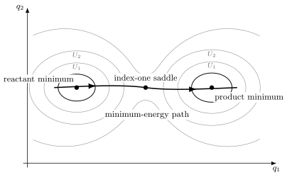
A two-coordinate slice of a molecular energy landscape. Minima define basins and an index-one saddle defines a local pass between them. The heavy curve is a minimum-energy path, not a claim about the time-dependent trajectory of a molecule. Real molecular surfaces have many more dimensions and may contain several competing passes.

Vibrational Motion Near a Minimum

Let $q_*$ be a nondegenerate minimum and write $\eta=q-q_*$. The local expansion is

$$\begin{aligned} U(q) ={}& U(q_*) +\frac12 \sum_{ij}K_{ij}\eta^i\eta^j \\ &+O(\lVert\eta\rVert^3). \end{aligned}$$

In mass-weighted Cartesian coordinates, the projected Hessian

$$\mathcal K = M^{-1/2}KM^{-1/2}$$

has internal eigenvectors $e_k$ satisfying

$$\mathcal K e_k = \omega_k^2e_k.$$

Positive eigenvalues give harmonic frequencies. The local nuclear Hamiltonian becomes a sum of oscillators,

$$H_{\mathrm{vib}}^{(2)} = \sum_{k=1}^{f} \left[ -\frac{\hbar^2}{2} \frac{\partial^2}{\partial Q_k^2} +\frac12\omega_k^2Q_k^2 \right],$$

with approximate energies

$$E_{\mathbf v} \approx U(q_*) +\sum_k \hbar\omega_k \left(v_k+\frac12\right).$$

This is the molecular realization of the oscillator as a universal local model. The approximation is local. Anharmonicity, mode coupling, torsion, inversion, dissociation, and tunneling probe higher derivatives and distant regions of the surface.

For a single bond coordinate, Vibrations of Diatomics turns this curvature into isotope-dependent levels, tests anharmonic and Morse descriptions, and shows why local constants do not uniquely determine dissociation.

At an index-one saddle, one projected Hessian eigenvalue is negative. Electronic-structure programs often report the corresponding $\omega^2<0$ direction as an imaginary frequency. That label diagnoses local negative curvature; it is not an oscillatory normal mode and does not by itself prove that the saddle connects the intended reactant and product.

Reaction Coordinates

A reaction coordinate is a function

$$\xi:\mathcal Q\longrightarrow\mathbb R$$

chosen to summarize progress through a process. It might be a bond-length difference, an angle, a collective variable, a path parameter, or a learned function. Its level set

$$\Sigma_{\xi_0} = \{q\in\mathcal Q:\xi(q)=\xi_0\}$$

contains all geometries assigned the same progress value.

Reducing a high-dimensional molecule to $\xi$ discards information. A good coordinate for plotting energy need not be a good coordinate for kinetics, and a coordinate that separates reactants from products need not resolve hidden intermediates or competing channels.

Paths through geometry space

A path is a curve

$$\gamma:[0,1]\longrightarrow\mathcal Q, \qquad s\longmapsto\gamma(s).$$

Its energy profile is the composition

$$U_\gamma(s)=U(\gamma(s)).$$

Different curves between the same basins generally give different profiles. The plotted profile is therefore not “the PES”; it is a one-dimensional restriction of the PES to a chosen curve.

Minimum-energy paths

For a path with unit tangent $\hat t(s)$ in a specified metric, a minimum-energy path satisfies

$$\left[ I-\hat t(s)\hat t(s)^{\mathsf T} \right] \operatorname{grad}U(\gamma(s)) =0.$$

The gradient has no component normal to the path. Its tangential component need not vanish. Chain-of-states algorithms such as the nudged elastic band and string methods approximate this condition with a discrete sequence of geometries.

A minimum-energy path is useful for finding passes and organizing local vibrational coordinates. It is not necessarily unique, globally lowest, or dynamically dominant.

Intrinsic reaction coordinates

The conventional intrinsic reaction coordinate, or IRC, follows mass-weighted steepest descent away from an index-one saddle. In mass-weighted coordinates $Q$,

$$\frac{dQ}{ds} = \mp \frac{\nabla_QU} {\lVert\nabla_QU\rVert}.$$

At the saddle the gradient is zero, so the integration is initialized by small displacements along the negative-curvature Hessian eigenvector in both directions. The two branches identify the minima reached by that local steepest-descent construction.

The IRC depends on the mass metric and on the surface used. Isotopic masses can therefore change the path parameterization and, in curvilinear coordinates, the path itself even when the Born–Oppenheimer energy surface is unchanged.

A path is not a trajectory

A classical trajectory obeys a second-order equation,

$$M\ddot R(t) = -\nabla_RU(R(t)),$$

and depends on initial positions and momenta. It can cross contour lines obliquely, oscillate across a valley, recross a dividing surface, or leave the neighborhood of a minimum-energy path.

A quantum nuclear wavepacket is more different still: it spreads, interferes, tunnels, and may occupy several electronic surfaces. A reaction path is geometric bookkeeping, whereas dynamics is evolution in phase space or Hilbert space.

Barriers and Transition States

For a reactant minimum $R_r$ and a connecting saddle $R^\ddagger$, the electronic barrier on one surface is

$$\Delta E_e^\ddagger = U(R^\ddagger)-U(R_r).$$

Several quantities are often called “the barrier”:

$$\begin{aligned} \Delta E_e^\ddagger &= \text{electronic energy difference}, \\ \Delta E_0^\ddagger &= \Delta E_e^\ddagger +\Delta E_{\mathrm{ZPE}}^\ddagger, \\ \Delta H^\ddagger(T) &= \text{activation enthalpy}, \\ \Delta G^\ddagger(T) &= \text{activation free energy}. \end{aligned}$$

They are not interchangeable. The first is a property of a specified PES; the others include nuclear and thermodynamic information.

Saddle point versus dynamical transition state

An index-one saddle is often called a transition structure. A transition state in rate theory is more fundamentally a dividing surface separating reactant and product regions in phase space. The best dividing surface need not pass through the lowest potential-energy saddle, especially for barrierless capture, entropic bottlenecks, roaming dynamics, strong recrossing, or reactions with several coupled coordinates.

Conventional transition-state theory gives

$$k_{\mathrm{TST}}(T) = \frac{k_BT}{h} \exp\left[ -\beta\Delta G^\ddagger(T) \right].$$

A dynamical correction is often written

$$k(T) = \kappa(T)k_{\mathrm{TST}}(T).$$

The interpretation of $\kappa$ depends on convention: recrossing, tunneling, nonadiabatic transitions, and nonequilibrium preparation may be separated or bundled differently. A barrier height alone is never a rate constant.

Barrierless does not mean structureless

If energy decreases monotonically along a chosen entrance path, the reaction is barrierless on that path. Long-range capture, angular-momentum barriers, zero-point constraints, narrow dynamical bottlenecks, and free-energy barriers can still control the rate. Conversely, quantum tunneling can produce reaction below a classical saddle energy.

Potential Energy and Free Energy

At temperature $T$, suppose all coordinates except a collective variable $\xi(q)$ are averaged in a classical canonical ensemble. A potential of mean force can be written

$$\begin{aligned} F(\xi) &= -k_BT\ln\mathcal Z(\xi)+C, \\ \mathcal Z(\xi) &= \int_{\mathcal Q}d\mu(q) \\ &\quad\times \delta\!\left(\xi(q)-\xi\right) e^{-\beta U(q)}. \end{aligned}$$

The measure $d\mu(q)$ contains the coordinate metric, constraints, and any Jacobian factors. Consequently:

• $F(\xi)$ depends on temperature and ensemble;
• it depends on the definition and normalization of $\xi$;
• it includes entropy from coordinates integrated out;
• it is not obtained by merely evaluating $U$ along one optimized path.

For quantum nuclei, the constrained object is defined through a density operator or path integral rather than the classical configurational integral above. Solvent, electronic excitations, and external fields can contribute further free-energy terms.

Entropic barriers

Imagine a valley with the local form

$$U(x,y) = V(x)+\frac12k(x)y^2.$$

Integrating over $y$ classically gives

$$F(x) = V(x) +\frac{k_BT}{2}\ln k(x) +C.$$

A narrow region with large $k(x)$ can therefore be a free-energy bottleneck even if $V(x)$ has no potential barrier. Energy landscapes and free-energy landscapes answer different questions.

Asymptotic Channels

A global reactive surface must describe more than stationary points. As fragments separate,

$$\begin{aligned} U(R) &\longrightarrow E_{\alpha}^{\mathrm{frag}} +V_{\alpha}^{\mathrm{long}}(R), \\ R &\longrightarrow\infty \quad \text{in channel }\alpha. \end{aligned}$$

where $\alpha$ labels a dissociation channel. The threshold $E_{\alpha}^{\mathrm{frag}}$ must be consistent with the electronic method used in the interaction region.

Long-range interactions can contain charge–charge, charge–dipole, induction, dispersion, and anisotropic multipole terms. A flexible interpolant that fits a finite cloud of points need not extrapolate to the correct power law. Size consistency, separated-fragment degeneracies, and channel energy ordering are essential validation targets.

Local surfaces designed for spectroscopy near one minimum need not be trusted for bond breaking. Conversely, a global reactive surface may sacrifice the sub-wavenumber accuracy required for precision spectroscopy. Domain and intended observables belong in the model specification.

Crossings and Conical Intersections

One scalar surface is inadequate when several electronic states become close. A local real two-state Hamiltonian can be written

$$W(R) = U_0(R)I +x(R)\sigma_z +y(R)\sigma_x.$$

Its adiabatic eigenvalues are

$$U_\pm(R) = U_0(R) \pm \sqrt{x(R)^2+y(R)^2}.$$

A degeneracy requires

$$x(R)=0, \qquad y(R)=0.$$

For a real electronic Hamiltonian, these are generically two independent conditions. In an $f$-dimensional internal space, conical intersections therefore form seams of dimension $f-2$. The two directions that lift the degeneracy are the branching plane. With a genuinely complex Hermitian two-state Hamiltonian, a $\sigma_y$ coefficient supplies a third condition, so the generic codimension changes.

The noncrossing rule in context

Along one tunable coordinate, two states of the same symmetry generically avoid crossing because one parameter cannot satisfy two independent degeneracy conditions. States protected from mixing by different exact symmetries may cross. In the full multidimensional nuclear space, same-symmetry conical-intersection seams are common because enough coordinates are available.

A one-dimensional scan can therefore be misleading:

• an avoided crossing in the scan may be a nearby conical intersection in the full space;
• a visible crossing may be symmetry protected;
• ordering states by energy can swap their electronic character.

Adiabatic and diabatic representations

The diagonal adiabatic representation makes energies simple but derivative couplings can become large or singular near a degeneracy. A smooth multistate model instead uses a matrix

$$\mathbf W(R) = \begin{pmatrix} W_{11}(R) & W_{12}(R)\\ W_{21}(R) & W_{22}(R) \end{pmatrix},$$

whose eigenvalues reproduce the adiabatic surfaces. Such a representation is usually called diabatic or quasi-diabatic. A strictly derivative-coupling-free diabatic basis need not exist globally; topology can obstruct it.

Adiabatic energies alone are insufficient for nonadiabatic dynamics. One also needs derivative couplings, a diabatic matrix with off-diagonal interactions, or equivalent gauge-covariant information. Born–Oppenheimer Berry Phase owns the sign change and geometric phase around a conical intersection.

A Solvable Two-Dimensional Landscape

Consider

$$U(x,y) = V_b \left( \frac{x^2}{a^2}-1 \right)^2 +\frac12ky^2,$$

with $V_b>0$, $a>0$, and $k>0$. The stationary equations are

$$\begin{aligned} \frac{\partial U}{\partial x} &= \frac{4V_bx}{a^2} \left( \frac{x^2}{a^2}-1 \right) =0, \\ \frac{\partial U}{\partial y} &=ky=0. \end{aligned}$$

There are minima at $(x,y)=(\pm a,0)$ and a saddle at $(0,0)$. The Hessian is

$$K(x,y) = \begin{pmatrix} \dfrac{4V_b}{a^2} \left( \dfrac{3x^2}{a^2}-1 \right) & 0 \\ 0 & k \end{pmatrix}.$$

At either minimum,

$$K_{\min} = \operatorname{diag} \left( \frac{8V_b}{a^2},k \right),$$

whereas at the central point,

$$K_{\ddagger} = \operatorname{diag} \left( -\frac{4V_b}{a^2},k \right).$$

The central point has index one. The minimum-energy path is $y=0$, and the electronic barrier is exactly

$$\Delta E_e^\ddagger=V_b.$$

If the kinetic energy is

$$T = \frac12m_x\dot x^2 +\frac12m_y\dot y^2,$$

the minimum frequencies are

$$\omega_x = \sqrt{\frac{8V_b}{m_xa^2}}, \qquad \omega_y = \sqrt{\frac{k}{m_y}}.$$

At the saddle, the unstable direction has

$$\omega_{\ddagger,x}^2 = -\frac{4V_b}{m_xa^2}.$$

This model separates several ideas cleanly: stationary-point index is determined by curvature, the path is geometric, the barrier is an energy difference, and the dynamical time scales require masses.

Computational Representation

Except for very small systems, a useful surface is reconstructed from finite electronic-structure data. A typical data set is

$$\begin{aligned} \mathcal O_n &= (E_n,\nabla E_n,\nabla^2E_n, \mathbf d_{ab,n},\ldots), \\ \mathcal D &= \{(R_n,\mathcal O_n)\}_{n=1}^{N}. \end{aligned}$$

Not every project contains every derivative or coupling. The representation should be designed around the intended observable: stationary structures need reliable gradients and Hessians, trajectories need smooth forces, spectroscopy needs delicate local curvature and anharmonicity, and scattering needs correct asymptotes.

Representation families

Family	Strengths and cautions
Grids, splines, and local polynomials	Transparent for low dimension; scale poorly and can misbehave outside the grid
Physically motivated analytic forms	Encode dissociation and long range; may be too rigid in complex reactive regions
Many-body expansions	Organize fragment limits; truncation and switching functions require care
Permutationally invariant polynomials	Enforce exchange symmetry exactly; basis size can grow rapidly
Reproducing kernels and Gaussian processes	Smooth interpolation and, for Gaussian processes, uncertainty estimates; kernels and asymptotes must be chosen deliberately
Neural and equivariant potentials	Flexible and scalable; extrapolation, data coverage, and physical constraints remain central
Diabatic matrix fits	Represent coupled surfaces and crossings; gauge consistency and off-diagonal data add difficulty

The phrase machine-learned potential identifies the regression strategy, not the underlying physical accuracy. A model trained on density-functional data reproduces that reference level plus fitting error; it does not silently become exact electronic structure.

Required invariances

For an isolated molecule, the fitted energy should satisfy

$$\widetilde U( \{\mathcal R\mathbf R_A+\mathbf a\} ) = \widetilde U( \{\mathbf R_A\} )$$

for every rigid rotation $\mathcal R$ and translation $\mathbf a$. Exchanging identical nuclei must also leave the energy unchanged:

$$\widetilde U(P R) = \widetilde U(R).$$

These properties may be built through internal coordinates, invariant descriptors, symmetrized polynomial bases, equivariant architectures followed by scalar readout, or explicit data augmentation. Exact architectural invariance is usually more reliable than hoping a finite training set teaches it everywhere.

Energy–force consistency

When forces are used for dynamics, they should derive from one scalar model:

$$\widetilde{\mathbf F}_A(R) = -\nabla_A\widetilde U(R).$$

This guarantees conservative forces within the modeled isolated system. Fitting independent force components without integrability can produce path-dependent work and energy drift.

A common joint objective is

$$\begin{aligned} \mathcal L(\theta) ={}& \mathcal L_E+\mathcal L_F +\mathcal R(\theta), \\ \mathcal L_E ={}& \sum_nw_E \lvert U_\theta(R_n)-E_n\rvert^2, \\ \mathcal L_F ={}& \sum_nw_F \lVert\nabla U_\theta(R_n)+\mathbf F_n\rVert^2. \end{aligned}$$

where $\mathcal R$ regularizes the representation. The weights define which errors the fit prioritizes; they are part of the model, not mere numerical decoration.

Sampling is the central problem

Configuration space grows rapidly with molecule size. Uniform grids become impossible, and equilibrium samples may miss transition states, repulsive walls, dissociation channels, rare conformers, and nonadiabatic regions.

A defensible sampling loop is:

1. define the chemical domain, electronic states, and target observables;
2. seed known minima, saddles, asymptotes, and distorted structures;
3. fit an initial representation;
4. explore with dynamics, path searches, normal-mode sampling, or uncertainty-guided queries;
5. recompute suspicious geometries at the reference electronic level;
6. repeat until observable-level validation is stable.

Active learning can reduce the number of expensive electronic calculations, but its uncertainty indicator must itself be calibrated. Committee disagreement or posterior variance can miss a shared model bias.

Validation and Uncertainty

A single root-mean-square test error is not enough. Large errors in a small but dynamically decisive region can be hidden by many easy near-equilibrium points.

What to validate

A surface intended for broad use should be tested on:

• energies on genuinely withheld configurations;
• forces and directional derivatives;
• equilibrium geometries and relative conformer energies;
• Hessians and harmonic frequencies;
• saddle locations, indices, and barrier heights;
• dissociation energies and long-range power laws;
• permutation and rigid-motion invariance;
• continuity across coordinate charts and switching regions;
• energy conservation in microcanonical trajectories;
• bound levels, scattering observables, or rates relevant to its stated purpose;
• robustness under new sampling outside the original trajectory ensemble.

Train/test splits made by randomly separating adjacent molecular-dynamics frames can overstate transferability because neighboring frames are strongly correlated. Splits by trajectory, basin, energy range, composition, or reaction channel are more revealing.

An uncertainty ledger

At least four error layers should be kept separate:

$$\begin{aligned} \delta_{\mathrm{total}} \sim &\; \delta_{\mathrm{Hamiltonian}} +\delta_{\mathrm{electronic}} \\ &+ \delta_{\mathrm{representation}} +\delta_{\mathrm{dynamics}}. \end{aligned}$$

• Hamiltonian error: neglected relativity, fields, environments, or finite-mass effects.
• Electronic-structure error: basis incompleteness, correlation truncation, functional error, and state-tracking failure.
• Representation error: finite data, regression bias, symmetry defects, and extrapolation.
• Dynamics error: classical nuclei, reduced dimensionality, semiclassical approximation, neglected nonadiabatic coupling, and sampling error.

Agreement with experiment tests the combined pipeline. Compensating errors can make one observable accurate while the surface remains unreliable elsewhere.

Reproducibility record

A reusable surface should publish:

• Hamiltonian, electronic method, basis sets, and software versions;
• state definitions and phase or diabatization conventions;
• coordinate and symmetry conventions;
• training geometries, energies, derivatives, units, and provenance;
• fit architecture, hyperparameters, loss weights, and random seeds;
• domain of intended use and explicit exclusions;
• validation sets and observable benchmarks;
• uncertainty or applicability diagnostics;
• a versioned evaluation implementation.

The data and executable representation are part of the scientific result. A plot and one aggregate error number are not enough for reproduction.

Common Mistakes

• Calling a one-dimensional scan “the potential energy surface.”
• Omitting the electronic state, energy zero, or internuclear-repulsion convention.
• Treating $R_e$ as the measured molecular structure without nuclear averaging.
• Counting Cartesian translations and rotations as vibrations.
• Calling every stationary point a transition state without checking Hessian index and connectivity.
• Assuming an imaginary frequency proves the intended reaction path.
• Equating a minimum-energy path with a classical trajectory or quantum wavepacket.
• Using an electronic barrier, zero-point-corrected barrier, and activation free energy interchangeably.
• Interpreting a barrierless PES as automatically fast dynamics.
• Inferring a conical intersection or its absence from one coordinate scan.
• Fitting adiabatic energies near a crossing without couplings or a multistate representation.
• Trusting interpolation error as an estimate of electronic-structure error.
• Validating energies while ignoring forces, Hessians, asymptotes, and target observables.
• Extrapolating a local spectroscopic surface into bond-breaking geometries.
• Treating a machine-learned potential as accurate outside its sampled chemical domain.

A Practical Reading Workflow

When encountering a published surface, ask in this order:

1. Which electronic Hamiltonian and states define it?
2. Is it Born–Oppenheimer, DBOC corrected, diabatic, free energetic, or empirical?
3. What geometry space and coordinate metric are used?
4. Which symmetries and asymptotic channels are enforced?
5. What electronic data and derivatives were fitted?
6. Where are the minima, saddles, crossings, and excluded regions?
7. Which observables were used for validation?
8. Which uncertainty layer dominates the intended application?

These questions turn a landscape picture into a scientific model with a stated domain of validity.

Connections

• Molecular Quantum Mechanics places surfaces within the chapter’s structure, bonding, and spectroscopy map.
• Molecular Hamiltonian defines the all-particle Coulomb problem from which the fixed-geometry electronic operator is obtained.
• Born–Oppenheimer in Molecules develops nuclear motion, isotope effects, and molecular accuracy on one or several surfaces.
• Nonadiabatic Coupling turns surface gaps, couplings, and representations into multistate molecular dynamics.
• Conical Intersections develops the local double-cone geometry, seam topology, geometric phase, and computational tests.
• Electronic Structure Overview compares and validates the electronic models used to construct each surface.
• Chemical Bonding distinguishes bound-state evidence and channel-specific dissociation energies from orbital, density, bond-order, and energy-decomposition interpretations.
• Rotations of Molecules connects equilibrium geometry and vibrational averaging to inertia tensors, rotational constants, distortion, and microwave structure inference.
• Vibrations of Diatomics connects one-dimensional surface curvature and global well shape to term values, isotope shifts, dissociation, and infrared transition moments.
• Normal Modes of Polyatomics turns a polyatomic Hessian into mass-weighted vibrational coordinates, symmetry labels, activities, and computational diagnostics.
• Electronic Spectroscopy distinguishes adiabatic, 0–0, vertical, and band-maximum energies and develops the resulting Franck–Condon envelopes.
• Born–Oppenheimer Approximation as Scale Separation gives the coupled-channel equations and nonadiabatic validity criteria.
• Born–Oppenheimer Berry Phase is the canonical home for molecular geometric phases around degeneracies.
• Molecular Physics maps rotational, vibrational, electronic, and permutation symmetries.
• Quantum Chemistry Roadmap provides a broader route through electronic structure and molecular dynamics.
• Quantum Chemistry References annotates textbooks and specialist sources.

References

• M. Born and R. Oppenheimer, “Zur Quantentheorie der Molekeln,” Annalen der Physik 389, 457–484 (1927), doi:10.1002/andp.19273892002.
• M. Born and K. Huang, Dynamical Theory of Crystal Lattices, Oxford University Press (1954), Chapters IV and V.
• H. Eyring, “The activated complex in chemical reactions,” Journal of Chemical Physics 3, 107–115 (1935), doi:10.1063/1.1749604.
• J. N. Murrell and K. J. Laidler, “Symmetries of activated complexes,” Transactions of the Faraday Society 64, 371–377 (1968), doi:10.1039/TF9686400371.
• K. Fukui, “Formulation of the reaction coordinate,” Journal of Physical Chemistry 74, 4161–4163 (1970), doi:10.1021/j100717a029.
• K. Fukui, “The path of chemical reactions: the IRC approach,” Accounts of Chemical Research 14, 363–368 (1981), doi:10.1021/ar00072a001.
• W. H. Miller, N. C. Handy, and J. E. Adams, “Reaction path Hamiltonian for polyatomic molecules,” Journal of Chemical Physics 72, 99–112 (1980), doi:10.1063/1.438959.
• D. G. Truhlar and B. C. Garrett, “Variational transition-state theory,” Accounts of Chemical Research 13, 440–448 (1980), doi:10.1021/ar50156a002.
• G. Henkelman, B. P. Uberuaga, and H. Jónsson, “A climbing image nudged elastic band method for finding saddle points and minimum energy paths,” Journal of Chemical Physics 113, 9901–9904 (2000), doi:10.1063/1.1329672.
• J. von Neumann and E. Wigner, “Über das Verhalten von Eigenwerten bei adiabatischen Prozessen,” Physikalische Zeitschrift 30, 467–470 (1929).
• E. Teller, “The crossing of potential surfaces,” Journal of Physical Chemistry 41, 109–116 (1937), doi:10.1021/j150379a010.
• H. C. Longuet-Higgins, U. Öpik, M. H. L. Pryce, and R. A. Sack, “Studies of the Jahn–Teller effect. II. The dynamical problem,” Proceedings of the Royal Society A 244, 1–16 (1958), doi:10.1098/rspa.1958.0022.
• C. A. Mead and D. G. Truhlar, “On the determination of Born–Oppenheimer nuclear motion wave functions including complications due to conical intersections and identical nuclei,” Journal of Chemical Physics 70, 2284–2296 (1979), doi:10.1063/1.437734.
• D. R. Yarkony, “Diabolical conical intersections,” Reviews of Modern Physics 68, 985–1013 (1996), doi:10.1103/RevModPhys.68.985.
• T.-S. Ho, T. Hollebeek, H. Rabitz, L. B. Harding, and G. C. Schatz, “A global H$_2$O potential energy surface for the reaction O($^1D$) + H$_2$ → OH + H,” Journal of Chemical Physics 105, 10472–10486 (1996), doi:10.1063/1.472977.
• H. Partridge and D. W. Schwenke, “The determination of an accurate isotope dependent potential energy surface for water from extensive ab initio calculations and experimental data,” Journal of Chemical Physics 106, 4618–4639 (1997), doi:10.1063/1.473987.
• Z. Xie and J. M. Bowman, “Permutationally invariant polynomial basis for molecular energy surface fitting via monomial symmetrization,” Journal of Chemical Theory and Computation 6, 26–34 (2010), doi:10.1021/ct9004917.
• T.-S. Ho and H. Rabitz, “Reproducing kernel Hilbert space interpolation methods as a paradigm of high dimensional model representations,” Journal of Chemical Physics 119, 6433–6442 (2003), doi:10.1063/1.1603219.
• J. Behler and M. Parrinello, “Generalized neural-network representation of high-dimensional potential-energy surfaces,” Physical Review Letters 98, 146401 (2007), doi:10.1103/PhysRevLett.98.146401.
• A. P. Bartók, M. C. Payne, R. Kondor, and G. Csányi, “Gaussian approximation potentials: the accuracy of quantum mechanics, without the electrons,” Physical Review Letters 104, 136403 (2010), doi:10.1103/PhysRevLett.104.136403.
• S. Chmiela, A. Tkatchenko, H. E. Sauceda, I. Poltavsky, K. T. Schütt, and K.-R. Müller, “Machine learning of accurate energy-conserving molecular force fields,” Science Advances 3, e1603015 (2017), doi:10.1126/sciadv.1603015.
• J. M. Bowman et al., “Ab initio-based potential energy surfaces for complex molecules and molecular complexes,” Journal of Physical Chemistry Letters 1, 1866–1874 (2010), doi:10.1021/jz100626h.

Exercises

1. Surface conventions

One calculation reports an electronic eigenvalue $\mathcal E(R)$ that excludes internuclear repulsion, while another reports $E(R)$ from a Hamiltonian that includes it. Relate the two surfaces and their forces.

Solution

The convention translation is

$$E(R) = \mathcal E(R)+V_{NN}(R).$$

Therefore

$$\mathbf F_A = -\nabla_AE = -\nabla_A\mathcal E -\nabla_AV_{NN}.$$

Comparing $\mathcal E$ directly with $E$ would omit a geometry-dependent term, not merely shift the energy zero.

2. Classify the stationary points

For

$$U(x,y) = (x^2-1)^2+2y^2,$$

find every stationary point, its index, and the barrier between the two minima.

Solution

The gradient is

$$\nabla U = \left( 4x(x^2-1),4y \right),$$

so the stationary points are $(\pm1,0)$ and $(0,0)$. The Hessian is

$$K = \operatorname{diag} \left( 12x^2-4,4 \right).$$

At $(\pm1,0)$ it is $\operatorname{diag}(8,4)$, so both points are minima of index zero. At $(0,0)$ it is $\operatorname{diag}(-4,4)$, so the point is an index-one saddle. Since $U(\pm1,0)=0$ and $U(0,0)=1$, the barrier is $1$ in the chosen energy units.

3. Coordinate changes and Hessian index

Explain why a nonlinear coordinate change can alter the ordinary Hessian away from a stationary point but cannot change the index of a nondegenerate stationary point.

Solution

For $q=q(Q)$,

$$\begin{aligned} H^{(Q)}_{\alpha\beta} = &J^i_{\ \alpha} H^{(q)}_{ij} J^j_{\ \beta} \\ &+ \frac{\partial U}{\partial q^i} \frac{\partial^2q^i} {\partial Q^\alpha\partial Q^\beta}. \end{aligned}$$

The second line is generally nonzero, so the ordinary Hessian is not a tensor away from stationarity. At a stationary point $\partial_iU=0$, leaving

$$H^{(Q)}=J^{\mathsf T}H^{(q)}J.$$

For nonsingular $J$, Sylvester’s law of inertia says that this congruence preserves the numbers of positive and negative eigenvalues. The index is therefore invariant.

4. Path versus trajectory

A minimum-energy path descends from a saddle to a reactant minimum. Must a classical trajectory launched near the saddle follow that curve? Give two reasons.

Solution

No. First, a minimum-energy path is defined by a first-order geometric condition on the gradient normal to the path, whereas a trajectory obeys the second-order Newton equation and carries momentum. A transverse initial velocity immediately moves the trajectory away from the path.

Second, the path is usually defined with a chosen mass or coordinate metric. Dynamics also depends on the full mass matrix and can exchange energy among transverse modes. Recrossing and valley oscillation are therefore possible even on a perfectly known surface.

5. Isotope substitution

In the solvable landscape, replace $m_x$ by $2m_x$ while leaving the electronic Hamiltonian unchanged. What happens to the Born–Oppenheimer barrier and the harmonic frequency $\omega_x$?

Solution

The clamped-nuclei surface and its barrier $V_b$ are independent of nuclear mass, so the Born–Oppenheimer barrier is unchanged. The frequency becomes

$$\omega_x' = \sqrt{ \frac{8V_b}{(2m_x)a^2} } = \frac{\omega_x}{\sqrt2}.$$

Zero-point corrections and tunneling rates therefore change even though the underlying Born–Oppenheimer landscape does not.

6. An entropic bottleneck

For

$$U(x,y) = V(x)+\frac12k(x)y^2,$$

integrate out $y$ in a classical canonical ensemble and show how a narrow valley alters the free-energy profile.

Solution

At fixed $x$,

$$\begin{aligned} Z_y(x) &= \int_{-\infty}^{\infty} dy\, e^{-\beta k(x)y^2/2} \\ &= \sqrt{ \frac{2\pi}{\beta k(x)} }. \end{aligned}$$

Hence

$$\begin{aligned} F(x) &= -k_BT\ln \left[ e^{-\beta V(x)}Z_y(x) \right] +C \\ &= V(x) +\frac{k_BT}{2}\ln k(x) +C'. \end{aligned}$$

Large $k(x)$ means a narrow transverse distribution and less configurational entropy. It raises $F(x)$ even if $V(x)$ is flat or decreasing.

7. Crossing codimension

For the real two-state matrix

$$W = U_0I+x\sigma_z+y\sigma_x,$$

derive the eigenvalue gap and explain why a generic conical-intersection seam has dimension $f-2$ in an $f$-dimensional nuclear space.

Solution

The eigenvalues are

$$U_\pm = U_0\pm\sqrt{x^2+y^2},$$

so the gap is

$$\Delta U = 2\sqrt{x^2+y^2}.$$

Degeneracy requires the two independent scalar conditions $x=0$ and $y=0$. Generically, each condition removes one dimension. Their simultaneous solution therefore has dimension $f-2$. The two transverse directions form the local branching plane.

8. Validate a reactive fit

A fitted surface has a test-set energy root-mean-square error of $0.2\ \mathrm{kcal\,mol^{-1}}$. List four additional checks needed before using it for a bond-breaking reaction.

Solution

Four essential checks are:

1. force errors on independently sampled geometries, especially near the reaction region;
2. saddle location, Hessian index, and barrier error against direct electronic calculations;
3. dissociation thresholds and the correct long-range asymptotic behavior;
4. dynamical validation such as energy conservation and convergence of reaction probabilities or rate coefficients.

One should also test permutation invariance, separated-fragment size consistency, coverage of alternative channels, and whether the electronic reference method itself is adequate for bond breaking. A small aggregate interpolation error cannot answer those questions.