Molecular Orbitals

A molecular orbital is a one-electron function used to represent electronic structure at a specified molecular geometry. It may be an exact eigenfunction for a genuine one-electron molecule, an eigenfunction of a mean-field operator such as the Hartree–Fock or Kohn–Sham operator, or a member of some other deliberately chosen one-particle basis. The word orbital therefore identifies a mathematical role only after the Hamiltonian, approximation, basis, geometry, and spin convention have been stated.

Molecular-orbital language is powerful because it turns a complicated electronic problem into a sequence of one-particle ideas: atom-centered functions mix, symmetry filters the allowed mixing, levels split, electrons occupy spin-orbitals, and the resulting configurations organize bonding and spectroscopy. The price is conceptual discipline. An orbital diagram is not the exact many-electron wavefunction, an orbital coefficient is not an observable, and a HOMO–LUMO separation is not automatically an excitation energy.

This page develops the molecular one-particle language. Atomic Orbitals Revisited owns the broader distinction among exact, Hartree–Fock, Kohn–Sham, natural, localized, and Dyson orbitals. Hartree–Fock Approximation owns the variational derivation of the self-consistent-field equations. Electronic Structure Overview places orbital bases inside Hartree–Fock, configuration-interaction, coupled-cluster, density-functional, multireference, and excited-state method choices. Molecular Orbital Computation provides a reproducible two-function H₂⁺ calculation of the overlap metric, generalized eigenproblem, and bonding–antibonding curves. Here the emphasis is how orbitals mix and are interpreted in molecules.

Canonical Scope

This page is the canonical home for:

• linear combinations of atom-centered basis functions and their overlap metric;
• bonding, antibonding, and nonbonding orbital language;
• homonuclear and heteronuclear two-center mixing;
• $\sigma$, $\pi$, and $\delta$ labels in linear molecules;
• orbital occupations, qualitative MO diagrams, and simple MO bond order;
• HOMO, LUMO, SOMO, frontier-orbital, and orbital-gap terminology;
• the distinction between canonical, localized, and exact many-electron descriptions;
• checks needed to interpret a computed molecular orbital reproducibly.

It does not derive the full molecular Coulomb operator, which belongs to Molecular Hamiltonian, or the electronic-channel approximation, which belongs to Born–Oppenheimer in Molecules. Valence Bond Theory owns localized spin-coupled structures, resonance, hybridization language, and the exact and truncated relations between MO and VB expansions. Detailed bond energetics require complete potential-energy surfaces, not a single orbital diagram. Chemical Bonding owns the broader stability criteria and the comparison of orbital bond order with density, force, spectroscopic, and decomposition diagnostics.

The Fixed-Geometry One-Particle Problem

Choose a nuclear geometry $R=\{\mathbf R_A\}$ and solve the clamped-nuclei electronic problem at that geometry. A molecular orbital is a function of one electron coordinate,

$$\phi_p(\mathbf r;R),$$

or, when spin is included explicitly, a spin-orbital

$$\chi_p(x;R), \qquad x=(\mathbf r,\sigma).$$

The geometry label matters. Changing a bond length or angle changes the electronic operator and therefore changes the orbitals, their ordering, and often their qualitative character.

Exact only for a one-electron electronic problem

For a one-electron molecular ion, the clamped-nuclei electronic equation has the form

$$\hat h_e(R)\phi_p(\mathbf r;R) = \epsilon_p(R)\phi_p(\mathbf r;R).$$

Apart from the stated nonrelativistic and fixed-nucleus approximations, $\phi_p$ can then be an exact electronic eigenstate.

For several electrons, the Coulomb interaction depends on pairs of coordinates,

$$\hat V_{ee} = \sum_{i<j}\frac{1}{r_{ij}},$$

so the exact state is a function

$$\Psi(x_1,\ldots,x_N;R),$$

not a list of independent one-electron wavefunctions. Hartree–Fock, Kohn–Sham density-functional theory, configuration-interaction expansions, Green-function methods, and reduced-density-matrix analyses introduce orbitals in different ways. The same plotted shape can therefore have different physical status in different calculations.

Three objects that should not be conflated

Object	Typical notation	What it means
atom-centered basis function	$\chi_\mu(\mathbf r)$	a chosen function used to span a finite one-particle space
molecular orbital	$\phi_p(\mathbf r)$	a linear combination or eigenfunction in that space
many-electron state	$\Psi(x_1,\ldots,x_N)$	the antisymmetric electronic state from which observables are calculated

An “atomic orbital” in an LCAO calculation is commonly an atom-centered Gaussian or numerical basis function. It need not be an exact eigenstate of an isolated atom. A contracted basis may contain several functions of the same angular character on one center, polarization functions absent from the isolated occupied shell, and diffuse functions designed to represent molecular tails.

Linear Combination of Atomic Orbitals

Let $\{\chi_\mu\}_{\mu=1}^{K}$ be linearly independent atom-centered basis functions. A molecular orbital is expanded as

$$\phi_p(\mathbf r) = \sum_{\mu=1}^{K} C_{\mu p}\chi_\mu(\mathbf r).$$

This is the linear combination of atomic orbitals, or LCAO, representation. The coefficients $C_{\mu p}$ say how the chosen basis functions combine. They are representation-dependent numbers; changing the basis changes the coefficients even when the represented function changes little.

The overlap matrix is the metric

Atom-centered functions on different nuclei are generally not orthogonal. Define

$$S_{\mu\nu} = \langle\chi_\mu|\chi_\nu\rangle.$$

For a normalized orbital with coefficient vector $\mathbf c_p$,

$$\langle\phi_p|\phi_p\rangle = \mathbf c_p^\dagger \mathbf S \mathbf c_p =1.$$

Mutual orthonormality of a set of molecular orbitals is

$$\mathbf C^\dagger \mathbf S \mathbf C = \mathbf I.$$

The matrix $\mathbf S$, not the Euclidean dot product of coefficient columns, supplies the inner product in a nonorthogonal basis. Thus $\sum_\mu |C_{\mu p}|^2=1$ is generally false.

Generalized secular equation

Let $\hat k$ be the one-particle operator being diagonalized. It might be an exact one-electron Hamiltonian, a converged Fock operator, or a Kohn–Sham operator. Define

$$K_{\mu\nu} = \langle\chi_\mu|\hat k|\chi_\nu\rangle.$$

Stationarity of the Rayleigh quotient

$$\mathcal R[\mathbf c] = \frac{ \mathbf c^\dagger\mathbf K\mathbf c }{ \mathbf c^\dagger\mathbf S\mathbf c }$$

gives

$$\mathbf K\mathbf c_p = \epsilon_p \mathbf S\mathbf c_p.$$

Collecting the eigenvectors gives the generalized matrix equation

$$\mathbf K\mathbf C = \mathbf S\mathbf C \boldsymbol{\varepsilon}.$$

This is an ordinary Hermitian eigenproblem only when $\mathbf S=\mathbf I$. If $\mathbf S$ is positive definite, a symmetric orthogonalization uses

$$\mathbf X = \mathbf S^{-1/2}, \qquad \mathbf X^\dagger \mathbf S \mathbf X = \mathbf I,$$

and transforms the problem to

$$\left( \mathbf X^\dagger \mathbf K \mathbf X \right) \mathbf C' = \mathbf C' \boldsymbol{\varepsilon}.$$

The back-transformed coefficients are $\mathbf C=\mathbf X\mathbf C'$.

Basis covariance and convergence

An invertible change among basis functions changes $\mathbf K$, $\mathbf S$, and $\mathbf C$ together while preserving the represented subspace and generalized eigenvalues. A coefficient attached to one primitive function is therefore not invariant. Even atom-by-atom populations require a specified partitioning prescription.

Near-linear dependence is a numerical warning. If $\mathbf S$ has a very small eigenvalue, some linear combination of basis functions has a very small norm. Orthogonalization then amplifies roundoff and integral error through $\mathbf S^{-1/2}$. Practical calculations monitor overlap eigenvalues, remove redundant combinations when justified, and test whether energies and observables are stable under basis changes.

Two Equivalent Centers

The smallest molecular-orbital calculation uses two normalized real functions $\chi_A$ and $\chi_B$ related by symmetry. Let

$$S = \langle\chi_A|\chi_B\rangle, \qquad |S|<1.$$

The normalized in-phase and out-of-phase combinations are

$$\phi_+ = \frac{ \chi_A+\chi_B }{ \sqrt{2(1+S)} },$$

and

$$\phi_- = \frac{ \chi_A-\chi_B }{ \sqrt{2(1-S)} }.$$

Their orthogonality follows directly from the symmetry-equivalent diagonal overlaps:

$$\langle\phi_+|\phi_-\rangle=0.$$

Energies in the two-function model

For a one-particle operator $\hat k$, define

$$\alpha = \langle\chi_A|\hat k|\chi_A\rangle = \langle\chi_B|\hat k|\chi_B\rangle,$$

and, after a real phase convention,

$$\beta = \langle\chi_A|\hat k|\chi_B\rangle.$$

The generalized eigenvalues are

$$E_\pm = \frac{ \alpha\pm\beta }{ 1\pm S }.$$

Their splitting is

$$E_--E_+ = \frac{ 2(\alpha S-\beta) }{ 1-S^2 }.$$

The in-phase combination is lower than the isolated diagonal level $\alpha$ precisely when

$$\beta<\alpha S.$$

Under the same condition, the out-of-phase combination lies above $\alpha$. This criterion is more informative than saying “overlap lowers the bonding orbital.” Overlap enters both the normalization and the Hamiltonian matrix element. The energetic result comes from their combination.

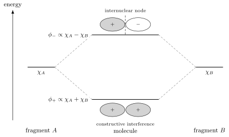
Two symmetry-equivalent atom-centered functions generate orthogonal in-phase and out-of-phase combinations. The lower combination has constructive amplitude between the centers in the usual bonding case; the upper combination has an internuclear node. The signs indicate relative wavefunction phase, not electric charge.

Interference in the density

For real basis functions,

$$|\phi_\pm(\mathbf r)|^2 = \frac{ |\chi_A|^2+|\chi_B|^2 \pm2\chi_A\chi_B }{ 2(1\pm S) }.$$

The cross term is the interference term. In a region where $\chi_A$ and $\chi_B$ have the same sign, it increases the in-phase density and decreases the out-of-phase density. A nodal surface appears wherever the amplitudes cancel.

Phase itself is conventional: replacing $\chi_B$ by $-\chi_B$ interchanges which algebraic combination is written with a plus sign. What is invariant is the spatial symmetry, nodal structure, density, and energy of each eigenfunction.

Why a node often raises the energy

A node forces stronger spatial variation. Through the kinetic operator,

$$\hat T = -\frac{\hbar^2}{2m_e}\nabla^2,$$

that variation often increases kinetic energy. Redistribution of density also changes electron–nuclear attraction, electron–electron repulsion in a many-electron model, and nuclear-screening effects. A molecular bond cannot generally be assigned to a single term without a specified energy-decomposition method.

The two-state algebra is the same as the Tight-Binding Dimer. The molecular application differs because the atom-centered basis is usually nonorthogonal and because the one-electron operator may be self-consistent.

H₂⁺ Ion applies this two-center algebra to an actual Coulomb Hamiltonian. It evaluates the overlap and Hamiltonian integrals in closed form, adds the proton–proton term to obtain potential curves, and compares the minimal basis with an accurate one-electron benchmark.

Hydrogen Molecule shows what changes when two electrons occupy the same orbital basis: a restricted $g^2$ determinant acquires ionic contamination at dissociation, while mixing $g^2$ and $u^2$ restores the neutral spin-singlet limit.

Unequal Centers and Polarized Orbitals

For a heteronuclear two-function illustration, first work in an orthonormal basis and choose phases so the coupling is $-t$ with $t\geq0$:

$$\mathbf K = \begin{pmatrix} \alpha_A & -t\\ -t & \alpha_B \end{pmatrix}.$$

Let

$$\Delta = \alpha_B-\alpha_A>0.$$

The eigenvalues are

$$E_{\mathrm{low,high}} = \frac{\alpha_A+\alpha_B}{2} \mp \sqrt{ \left(\frac{\Delta}{2}\right)^2+t^2 }.$$

A convenient parametrization of the lower eigenvector is

$$|\phi_{\mathrm{low}}\rangle = \cos\theta\,|A\rangle +\sin\theta\,|B\rangle,$$

where

$$\tan(2\theta) = \frac{2t}{\Delta}, \qquad 0\leq\theta\leq\frac{\pi}{4}.$$

The upper eigenvector is the orthogonal combination

$$|\phi_{\mathrm{high}}\rangle = -\sin\theta\,|A\rangle +\cos\theta\,|B\rangle.$$

Two tests control the interpretation:

• Symmetry compatibility: only basis functions belonging to compatible symmetry sectors can mix.
• Energy matching: mixing is strong when $t$ is comparable to the diagonal mismatch $\Delta$ and weak when $t\ll\Delta$.

When $\Delta\gg t$, the lower orbital is concentrated on the lower-energy center and the upper orbital on the higher-energy center. When $\Delta\to0$, both approach equal-weight combinations. This is the one-particle origin of orbital polarization in a heteronuclear bond, but partial charge and dipole moment require the occupied many-electron density, not one coefficient squared.

In a nonorthogonal basis, the same physics is obtained from

$$\det( \mathbf K-E\mathbf S )=0.$$

Ignoring $\mathbf S$ changes both the eigenvalues and normalization and can produce a qualitatively wrong mixing analysis.

Bonding, Antibonding, and Nonbonding

The three labels describe how occupation of an orbital affects a stated molecular interaction within a stated model.

Label	Typical signature	Interpretation and qualification
bonding	constructive amplitude in an internuclear region	occupation tends to stabilize shorter separation, but this must be tested against a dissociation reference or energy derivative
antibonding	destructive amplitude with an additional node	occupation tends to oppose the corresponding bond; the asterisk is not a universal symmetry quantum number
nonbonding	weak coupling to the partner fragment	occupation has a relatively small first-order effect on that bond but may still polarize, hybridize, or affect other bonds

A label is relative to a coordinate

An orbital can be bonding with respect to one internuclear distance and antibonding with respect to another. In a polyatomic molecule, a delocalized orbital may stabilize one set of contacts while destabilizing another. A robust local diagnostic asks how an orbital contribution or occupied state changes as the relevant nuclear coordinate is varied.

For an orbital eigenvalue model, one sometimes examines

$$\frac{\partial\epsilon_p}{\partial R}.$$

Even that derivative is method-dependent and is not by itself the derivative of the total molecular energy. Nuclear repulsion, all occupied orbitals, relaxation, and correlation contribute to the physical force.

The simple MO bond-order index

For a diagram with clearly paired bonding and antibonding levels, the elementary index is

$$b_{\mathrm{MO}} = \frac{ N_{\mathrm b}-N_{\mathrm{ab}} }{2}.$$

Two electrons in a bonding level and none in its antibonding partner give $b_{\mathrm{MO}}=1$; equal populations give zero. This is a useful bookkeeping rule in minimal models. It is not a unique observable or a universal definition of chemical bond order. Basis choice, delocalization, correlation, orbital relaxation, and the choice of which levels form a pair all matter.

Population analyses, density-based indices, valence-bond weights, and energy decompositions answer related but different questions. Numerical bond orders should therefore be reported with their definition and method.

Sigma, Pi, and Delta Orbitals

For a linear molecule, choose the internuclear axis as $z$. In the ideal cylindrically symmetric clamped-nuclei problem, the projection of one-electron orbital angular momentum on the axis can label an orbital. If

$$\hat L_z\phi_\lambda = \hbar\lambda\phi_\lambda,$$

then the magnitude

$$\Lambda=|\lambda|$$

is denoted

$$\Lambda = 0,1,2,3,\ldots \quad\longleftrightarrow\quad \sigma,\pi,\delta,\phi,\ldots$$

for one-electron orbitals. Uppercase $\Sigma,\Pi,\Delta,\ldots$ usually label the projection of the total electronic orbital angular momentum of an electronic term. An orbital label and a many-electron term label are not interchangeable.

Sigma orbitals

A $\sigma$ orbital has $\Lambda=0$ and is invariant under rotation about the molecular axis, apart from its trivial phase. Atom-centered $s$ functions and $p_z$ functions can contribute to a $\sigma$ block when the axis is $z$. The label says nothing by itself about bonding:

$$\sigma, \qquad \sigma^*$$

may denote bonding and antibonding members of a qualitative pair, but both have $\sigma$ axial character.

Pi and higher axial character

A $\pi$ orbital has $\Lambda=1$. In a cylindrically symmetric problem, the $\lambda=+1$ and $\lambda=-1$ functions are degenerate. Real $\pi_x$ and $\pi_y$ orbitals are unitary combinations of those complex eigenfunctions and span the same two-dimensional subspace.

Similarly, $\delta$ denotes $\Lambda=2$. Bending a linear molecule or placing it in an anisotropic environment lowers the symmetry and can split or mix components according to the remaining point group.

Inversion and reflection labels are independent

For a centrosymmetric molecule, inversion through the center gives an additional parity label:

$$\hat i\phi = \begin{cases} +\phi, & g\ \text{(gerade)},\\ -\phi, & u\ \text{(ungerade)}. \end{cases}$$

The $g/u$ label is not the same as bonding/antibonding. For example, whether an in-phase combination is $g$ or $u$ depends on the intrinsic parity and orientation of the contributing atom-centered functions.

For a many-electron $\Sigma$ term, a superscript $+$ or $-$ can specify reflection symmetry in a plane containing the molecular axis. That sign also does not mean bonding or antibonding.

Polyatomic molecules

In a nonlinear molecule, point-group irreducible representations replace the continuous axial label. Matrix elements between basis functions of incompatible irreducible representations vanish when the operator respects the symmetry. The secular problem therefore block-diagonalizes:

$$\mathbf K = \bigoplus_\Gamma \mathbf K^{(\Gamma)}.$$

Only functions within compatible symmetry blocks can mix. Low symmetry permits more mixing; it does not guarantee strong mixing, because energetic mismatch can still suppress it. Molecular Symmetry develops character reduction, projection operators, and symmetry-adapted orbital combinations; Symmetry Applications to Molecular Physics supplies the wider application map.

How to Build and Read an MO Diagram

A qualitative diagram is a compressed model of a matrix eigenproblem. A disciplined construction follows these steps:

1. Choose the molecular geometry and the fragment partition.
2. Choose the atom-centered or fragment orbitals retained in the model.
3. Place fragment levels using a stated energy convention.
4. Sort functions by spin and spatial symmetry.
5. Couple only symmetry-compatible levels.
6. Estimate mixing strength from coupling and energy mismatch.
7. Order the resulting molecular levels.
8. Fill spin-orbitals subject to the Pauli principle and the chosen mean-field model.
9. Determine the many-electron spin and spatial symmetry; do not infer it from one orbital label alone.
10. Check the diagram against a computed spectrum, density, dissociation limit, or other target observable.

The vertical scale is often only qualitative. A line in a hand-drawn diagram may stand for an exact one-electron energy, a Hartree–Fock eigenvalue, a Kohn–Sham eigenvalue, an empirical ionization parameter, or no calibrated energy at all.

Occupations and spin

For orthonormal spin-orbitals, the Pauli principle permits occupation number zero or one. In a restricted closed-shell spatial-orbital model, two electrons of opposite spin occupy each spatial orbital. The density is then

$$\rho(\mathbf r) = 2\sum_{i\in\mathrm{occ}} |\phi_i(\mathbf r)|^2.$$

In an unrestricted or open-shell model, separate spin densities are needed:

$$\rho_\alpha(\mathbf r) = \sum_{i\in\alpha\mathrm{\ occ}} |\phi_i^\alpha(\mathbf r)|^2,$$ $$\rho_\beta(\mathbf r) = \sum_{j\in\beta\mathrm{\ occ}} |\phi_j^\beta(\mathbf r)|^2.$$

The total density and spin density are

$$\rho=\rho_\alpha+\rho_\beta, \qquad m_s=\rho_\alpha-\rho_\beta.$$

Degenerate or nearly degenerate levels require care. Filling them to maximize spin may be a useful first model, but the actual state ordering depends on electron repulsion, symmetry, spin–orbit interaction, vibronic coupling, and correlation.

A configuration is not yet an electronic state

An occupation string such as

$$(\sigma_g)^2(\sigma_u^*)^0$$

specifies a configuration in a chosen orbital basis. It does not by itself specify all spin couplings, spatial symmetry, or configuration mixing. Several symmetry-adapted states can arise from the same open-shell occupation pattern.

Slater Determinants owns the antisymmetric construction. A determinant built from occupied spin-orbitals is

$$\Phi(x_1,\ldots,x_N) = \frac{1}{\sqrt{N!}} \det[ \chi_i(x_j) ].$$

That determinant is a many-electron wavefunction. The orbital diagram is only a compact specification of the one-particle ingredients used to build it.

Canonical and Localized Molecular Orbitals

Canonical Hartree–Fock orbitals diagonalize the converged Fock operator,

$$\hat f|\phi_p\rangle = \epsilon_p|\phi_p\rangle.$$

They are often delocalized and symmetry-adapted. Let the occupied projector be

$$\hat P_{\mathrm{occ}} = \sum_{i=1}^{N_{\mathrm{occ}}} |\phi_i\rangle\langle\phi_i|.$$

For any unitary matrix $\mathbf U$ acting within the occupied subspace,

$$|\widetilde\phi_a\rangle = \sum_i|\phi_i\rangle U_{ia},$$

and

$$\sum_a |\widetilde\phi_a\rangle \langle\widetilde\phi_a| = \hat P_{\mathrm{occ}}.$$

The determinant changes only by the overall phase $\det\mathbf U$. Its density and Hartree–Fock energy do not change.

Localized bond and lone-pair orbitals exploit this freedom by optimizing a localization criterion. Boys, Edmiston–Ruedenberg, and Pipek–Mezey orbitals generally differ. None is the uniquely correct set of bonds hidden beneath the canonical solution. Each is a chosen basis for a subspace, useful when its criterion matches the question.

Rotations that mix occupied and virtual orbitals are different: they generally change the determinant and its energy. Likewise, rotating nondegenerate canonical orbitals produces functions that no longer diagonalize the Fock operator, even though they may span the same selected space.

Orbital Energies

An orbital energy has meaning only relative to the operator that generated it.

Orbital construction	Meaning of $\epsilon_p$	What it is not automatically
exact one-electron molecule	eigenvalue of the clamped-nuclei one-electron Hamiltonian	a full rovibronic transition energy
canonical Hartree–Fock	Lagrange-multiplier eigenvalue of the converged Fock operator	an exact removal, addition, or neutral excitation energy
Kohn–Sham	eigenvalue of an auxiliary density-reproducing system	a generic quasiparticle spectrum
localized or natural orbital	no unique energy unless an extra operator or convention is supplied	an eigenstate energy merely because the orbital is plotted

Hartree–Fock eigenvalues are not additive

In an orthonormal spin-orbital notation,

$$\epsilon_i = h_{ii} +\sum_{j\in\mathrm{occ}} \left( J_{ij}-K_{ij} \right).$$

The electronic Hartree–Fock energy is

$$E_{\mathrm{HF}} = \sum_{i\in\mathrm{occ}}h_{ii} + \frac12 \sum_{i,j\in\mathrm{occ}} \left( J_{ij}-K_{ij} \right).$$

Therefore

$$E_{\mathrm{HF}} = \sum_{i\in\mathrm{occ}}\epsilon_i - \frac12 \sum_{i,j\in\mathrm{occ}} \left( J_{ij}-K_{ij} \right).$$

A naive sum of occupied orbital energies double-counts the mean electron–electron interaction. Internuclear repulsion must also be added for the fixed-geometry molecular energy when it is not included in the electronic Hamiltonian convention.

Koopmans’ frozen-orbital statement

For canonical Hartree–Fock orbitals, removing an electron from occupied orbital $i$ without allowing any other orbital to relax gives

$$I_i^{\mathrm{frozen}} \approx -\epsilon_i^{\mathrm{HF}}.$$

This is Koopmans’ approximation. Orbital relaxation, electron correlation, different ionic-state mixing, relativistic effects, and nuclear motion modify the measured ionization energy. Virtual Hartree–Fock eigenvalues have no equally direct general interpretation as electron affinities.

HOMO, LUMO, and Frontier Language

For a specified one-particle spectrum:

• HOMO means the highest occupied molecular orbital;
• LUMO means the lowest unoccupied molecular orbital;
• SOMO means a singly occupied molecular orbital in an open-shell description;
• frontier orbitals usually means orbitals near the occupation boundary that dominate a chosen low-energy interaction or reactivity model.

These labels depend on electron number, geometry, spin treatment, charge state, external field, method, and basis. In an unrestricted calculation there can be separate $\alpha$ and $\beta$ frontier levels. Degeneracy may produce a frontier subspace rather than one unique orbital.

Three gaps that must be separated

The orbital gap is

$$\Delta_{\mathrm{orb}} = \epsilon_{\mathrm{LUMO}} - \epsilon_{\mathrm{HOMO}}.$$

The exact fundamental charge gap is

$$\begin{aligned} E_g &= I-A \\ &= E_0(N-1) + E_0(N+1) - 2E_0(N). \end{aligned}$$

A neutral excitation energy is

$$\Omega_n = E_n(N)-E_0(N).$$

An optical absorption onset additionally depends on transition matrix elements, selection rules, temperature, line broadening, and nuclear motion. In general,

$$\Delta_{\mathrm{orb}}, \qquad E_g, \qquad \Omega_n$$

are different quantities.

For exact ground-state Kohn–Sham theory under the standard assumptions, the fundamental gap can be written

$$E_g = \Delta_{\mathrm{KS}} + \Delta_{\mathrm{xc}},$$

where $\Delta_{\mathrm{xc}}$ is the exchange-correlation derivative discontinuity. Approximate functionals and generalized Kohn–Sham schemes require their own interpretation. A small computed HOMO–LUMO gap is therefore a warning about low-energy orbital rearrangement, not a universal measured excitation energy.

Frontier-orbital reasoning

Frontier-orbital theory asks whether an occupied orbital of one reactant and an unoccupied orbital of another:

• have compatible symmetry;
• overlap in the reacting region;
• have a favorable energy separation;
• retain the assumed character along the reaction coordinate.

This can organize trends and selection rules. It does not replace a potential-energy surface, transition-state calculation, solvent model, spin analysis, or nonadiabatic treatment. A reaction is governed by the total many-electron energy and dynamics, not by the visual proximity of two orbital lines.

Molecular Orbitals Versus Exact Many-Electron States

A correlated electronic eigenstate can be expanded in determinants,

$$|\Psi\rangle = \sum_I C_I|\Phi_I\rangle.$$

The orbitals and configuration coefficients together define the representation. A unitary change of the complete one-particle basis changes the determinant expansion but not the exact vector represented by a full configuration-interaction expansion.

The one-body reduced density matrix

For a normalized $N$-electron state, the spin-orbital one-body density matrix is

$$\begin{aligned} \gamma(x,x') ={}& N\int dx_2\cdots dx_N\, \\ &\times \Psi(x,x_2,\ldots,x_N) \\ &\times \Psi^*(x',x_2,\ldots,x_N). \end{aligned}$$

Its diagonal gives the one-electron density,

$$\rho(x)=\gamma(x,x).$$

Natural spin-orbitals diagonalize $\gamma$:

$$\int dx'\, \gamma(x,x') \varphi_k(x') = n_k\varphi_k(x),$$

with

$$0\leq n_k\leq1, \qquad \sum_k n_k=N.$$

A single determinant has $N$ occupation numbers equal to one and all others zero. Fractional natural occupations diagnose departure from a single determinant, although no single scalar captures every form of correlation. The canonical formalism belongs to Reduced Density Matrices.

State-specific removal amplitudes

Photoelectron observables are often better connected to a Dyson orbital, which overlaps an $N$-electron state with a specified $(N-1)$-electron ionic state:

$$\phi_D^{(a)}(x) = \sqrt N \int dX\, \Psi_{N-1}^{(a)*}(X) \Psi_N(x,X).$$

This is a transition amplitude between two many-electron states, not proof that a particular electron permanently occupied a visible orbital. Different ionic channels have different Dyson orbitals and removal energies.

Photoelectron Spectroscopy shows how those channel-specific overlaps enter measured electron energies, intensities, satellites, and angular distributions.

What remains invariant

Depending on the theory, robust content may include:

• total energies and energy differences;
• total electron and spin densities;
• transition amplitudes and response functions;
• symmetry quantum numbers of exact states;
• occupied projectors for a single determinant;
• natural occupation eigenvalues;
• poles and spectral weights of appropriate Green functions.

Individual canonical or localized orbital shapes are useful representations, but they are not universal observables. An experiment can constrain an orbital-like amplitude only through a specified forward model.

Worked Example: Heteronuclear Two-Level Mixing

Consider the orthonormal matrix, in electronvolts,

$$\mathbf K = \begin{pmatrix} -12 & -1.5\\ -1.5 & -8 \end{pmatrix}.$$

Here

$$\Delta=4, \qquad t=1.5.$$

The eigenvalues are

$$\begin{aligned} E_{\mathrm{low,high}} &= -10 \mp \sqrt{2^2+1.5^2} \\ &= -10\mp2.5, \end{aligned}$$

so

$$E_{\mathrm{low}}=-12.5\ \mathrm{eV}, \qquad E_{\mathrm{high}}=-7.5\ \mathrm{eV}.$$

The mixing angle satisfies

$$\tan(2\theta)=\frac{3}{4},$$

which gives

$$\theta\approx18.4^\circ.$$

The lower-orbital weights in this orthonormal two-function model are

$$\cos^2\theta=0.90, \qquad \sin^2\theta=0.10.$$

The lower orbital is therefore strongly polarized toward the lower-energy fragment function. Coupling stabilizes it by $0.5\ \mathrm{eV}$ relative to $\alpha_A$ and destabilizes the upper level by the same amount relative to $\alpha_B$.

This calculation does not imply a $0.90e$ charge on fragment $A$. Charge requires the occupations of all relevant orbitals, the overlap metric if the basis is nonorthogonal, and an explicitly chosen real-space or population partition.

A Reproducible Orbital Checklist

Before interpreting an orbital plot or table, record:

1. Geometry: nuclear coordinates, charge, multiplicity, and external fields.
2. Electronic method: one-electron model, Hartree–Fock variant, density functional, correlated method, or quasiparticle construction.
3. Basis and representation: atom-centered basis, pseudopotential, numerical grid, relativistic spinor convention, and linear-dependence threshold.
4. Orbital type: canonical, localized, natural, Dyson, corresponding, active-space, or another defined construction.
5. Spin and symmetry: restricted or unrestricted treatment, point group, irreducible representation, degeneracy, and phase convention where relevant.
6. Occupation convention: spin-orbital occupations, spatial occupations, fractional smearing, ensemble, or state averaging.
7. Rendered quantity: signed amplitude, density, difference density, transition density, current, or isosurface threshold.
8. Energy convention: operator, reference zero, electron number, and whether nuclear repulsion is included.
9. Convergence: basis, grid, self-consistency, stability, correlation space, and geometry sensitivity.
10. Observable connection: which energy, spectrum, force, density, or response the orbital analysis is intended to explain.

Two plots can look similar while representing different objects. Conversely, canonical and localized plots can look very different while representing the same occupied Hartree–Fock determinant.

Common Mistakes

• Treating an atom-centered basis function as an exact isolated-atom eigenstate. Basis functions are chosen variational ingredients.
• Normalizing nonorthogonal coefficients with an ordinary dot product. The correct norm is $\mathbf c^\dagger\mathbf S\mathbf c$.
• Reading orbital lobe signs as positive and negative charge. They represent relative phase; density is nonnegative.
• Saying overlap alone causes bonding. The energy depends on Hamiltonian and overlap matrix elements together.
• Assuming in-phase always means gerade. Inversion parity also depends on the intrinsic transformation of the contributing functions.
• Equating $\sigma$ with bonding and $\pi$ with antibonding. These are axial-symmetry labels; either sector can contain bonding and antibonding orbitals.
• Treating an MO configuration as the exact electronic state. Spin coupling, symmetry adaptation, and configuration interaction remain.
• Adding occupied Hartree–Fock eigenvalues to obtain the total energy. That double-counts the mean electron–electron interaction.
• Calling every HOMO–LUMO gap an optical gap. Orbital, fundamental, and neutral excitation gaps are distinct.
• Assigning partial charges from one coefficient squared. The result depends on overlap, occupations, and the partitioning method.
• Assuming canonical orbitals are unique chemical bonds. Occupied unitary rotations preserve the determinant and density.
• Interpreting virtual orbitals as empty states waiting unchanged for an electron. Addition and excitation reorganize the electronic state.
• Ignoring geometry. Orbital character and ordering can change along a reaction or distortion coordinate.
• Using orbital pictures without method metadata. A reproducible claim needs the operator, basis, spin, symmetry, and plotting convention.

References

1. J. E. Lennard-Jones, “The Electronic Structure of Some Diatomic Molecules,” Transactions of the Faraday Society 25, 668–686 (1929), doi:10.1039/TF9292500668.
2. R. S. Mulliken, “Electronic Structures of Polyatomic Molecules and Valence,” Physical Review 40, 55–62 (1932), doi:10.1103/PhysRev.40.55.
3. R. S. Mulliken, “Electronic Structures of Polyatomic Molecules and Valence. II. General Considerations,” Physical Review 41, 49–71 (1932), doi:10.1103/PhysRev.41.49.
4. C. C. J. Roothaan, “New Developments in Molecular Orbital Theory,” Reviews of Modern Physics 23, 69–89 (1951), doi:10.1103/RevModPhys.23.69.
5. T. Koopmans, “Über die Zuordnung von Wellenfunktionen und Eigenwerten zu den einzelnen Elektronen eines Atoms,” Physica 1, 104–113 (1934), doi:10.1016/S0031-8914(34)90011-2.
6. P.-O. Löwdin, “Quantum Theory of Many-Particle Systems. I. Physical Interpretations by Means of Density Matrices, Natural Spin-Orbitals, and Convergence Problems in the Method of Configurational Interaction,” Physical Review 97, 1474–1489 (1955), doi:10.1103/PhysRev.97.1474.
7. S. F. Boys, “Construction of Some Molecular Orbitals to Be Approximately Invariant for Changes from One Molecule to Another,” Reviews of Modern Physics 32, 296–299 (1960), doi:10.1103/RevModPhys.32.296.
8. C. Edmiston and K. Ruedenberg, “Localized Atomic and Molecular Orbitals,” Reviews of Modern Physics 35, 457–465 (1963), doi:10.1103/RevModPhys.35.457.
9. W. Kohn and L. J. Sham, “Self-Consistent Equations Including Exchange and Correlation Effects,” Physical Review 140, A1133–A1138 (1965), doi:10.1103/PhysRev.140.A1133.
10. J. F. Janak, “Proof That $\partial E/\partial n_i=\epsilon_i$ in Density-Functional Theory,” Physical Review B 18, 7165–7168 (1978), doi:10.1103/PhysRevB.18.7165.
11. J. P. Perdew and M. Levy, “Physical Content of the Exact Kohn–Sham Orbital Energies: Band Gaps and Derivative Discontinuities,” Physical Review Letters 51, 1884–1887 (1983), doi:10.1103/PhysRevLett.51.1884.
12. L. J. Sham and M. Schlüter, “Density-Functional Theory of the Energy Gap,” Physical Review Letters 51, 1888–1891 (1983), doi:10.1103/PhysRevLett.51.1888.
13. K. Fukui, T. Yonezawa, and H. Shingu, “A Molecular Orbital Theory of Reactivity in Aromatic Hydrocarbons,” Journal of Chemical Physics 20, 722–725 (1952), doi:10.1063/1.1700523.
14. J. Pipek and P. G. Mezey, “A Fast Intrinsic Localization Procedure Applicable for ab initio and Semiempirical Linear Combination of Atomic Orbital Wave Functions,” Journal of Chemical Physics 90, 4916–4926 (1989), doi:10.1063/1.456588.
15. A. I. Krylov, “From Orbitals to Observables and Back,” Journal of Chemical Physics 153, 080901 (2020), doi:10.1063/5.0018597.
16. A. Szabo and N. S. Ostlund, Modern Quantum Chemistry: Introduction to Advanced Electronic Structure Theory (Dover, 1996), Chapters 2–3.
17. T. Helgaker, P. Jørgensen, and J. Olsen, Molecular Electronic-Structure Theory (Wiley, 2000), Chapters 2, 10, and 11, doi:10.1002/9781119019572.
18. R. McWeeny, Methods of Molecular Quantum Mechanics, 2nd ed. (Academic Press, 1992), Chapters 3–6.
19. P. W. Atkins and R. S. Friedman, Molecular Quantum Mechanics, 5th ed. (Oxford University Press, 2011), Chapters 8–10.
20. I. N. Levine, Quantum Chemistry, 7th ed. (Pearson, 2014), Chapters 8–15.
21. F. A. Cotton, Chemical Applications of Group Theory, 3rd ed. (Wiley, 1990), Chapters 3–9.
22. G. Herzberg, Molecular Spectra and Molecular Structure. I. Spectra of Diatomic Molecules, 2nd ed. (Van Nostrand, 1950), Chapters I–III.

Exercises

1. Normalize two nonorthogonal combinations

Let $\chi_A$ and $\chi_B$ be normalized real functions with overlap $S$. Find normalization constants for

$$\psi_\pm = N_\pm \left( \chi_A\pm\chi_B \right),$$

and show that $\psi_+$ and $\psi_-$ are orthogonal when the two diagonal overlaps are equal.

Solution

Normalization gives

$$\begin{aligned} 1 &= N_\pm^2 \langle \chi_A\pm\chi_B | \chi_A\pm\chi_B \rangle \\ &= N_\pm^2 \left[ 2\pm2S \right]. \end{aligned}$$

Therefore

$$N_\pm = \frac{1}{\sqrt{2(1\pm S)}}.$$

The cross overlap is

$$\begin{aligned} \langle\psi_+|\psi_-\rangle &= N_+N_- \left( 1-S+S-1 \right) \\ &=0. \end{aligned}$$

The cancellation relies on equal diagonal norms and symmetric cross overlaps.

2. Derive the two-center energies

Using

$$\mathbf K = \begin{pmatrix} \alpha & \beta\\ \beta & \alpha \end{pmatrix}, \qquad \mathbf S = \begin{pmatrix} 1 & S\\ S & 1 \end{pmatrix},$$

derive $E_\pm$ and determine when the in-phase state lies below $\alpha$.

Solution

The generalized secular determinant is

$$\det \begin{pmatrix} \alpha-E & \beta-ES\\ \beta-ES & \alpha-E \end{pmatrix} =0.$$

It factors as

$$\begin{aligned} 0 ={}& \left[ \alpha+\beta-E(1+S) \right] \\ &\times \left[ \alpha-\beta-E(1-S) \right]. \end{aligned}$$

Thus

$$E_+ = \frac{\alpha+\beta}{1+S}, \qquad E_- = \frac{\alpha-\beta}{1-S}.$$

Since $1+S>0$,

$$E_+<\alpha$$

is equivalent to

$$\alpha+\beta < \alpha(1+S),$$

or

$$\beta<\alpha S.$$

The same condition gives $E_->\alpha$.

3. Explore heteronuclear mixing

For

$$\mathbf K = \begin{pmatrix} \alpha_A & -t\\ -t & \alpha_B \end{pmatrix}, \qquad \Delta=\alpha_B-\alpha_A>0,$$

show that the lower-state weight on $A$ is

$$w_A = \frac12 \left[ 1+ \frac{\Delta}{ \sqrt{\Delta^2+4t^2} } \right].$$

Evaluate the limits $t/\Delta\to0$ and $\Delta/t\to0$.

Solution

With

$$\tan(2\theta)=\frac{2t}{\Delta},$$

one has

$$\cos(2\theta) = \frac{\Delta}{ \sqrt{\Delta^2+4t^2} }.$$

Because the lower state is

$$|\phi_{\mathrm{low}}\rangle = \cos\theta|A\rangle +\sin\theta|B\rangle,$$

its $A$ weight is

$$w_A = \cos^2\theta = \frac{1+\cos(2\theta)}{2},$$

which gives the stated result. If $t/\Delta\to0$, then $w_A\to1$: the state localizes on the lower-energy center. If $\Delta/t\to0$, then $w_A\to1/2$: equivalent centers give equal mixing.

4. Separate axial, inversion, and bonding labels

For a centrosymmetric linear molecule, explain why each of the following statements is false:

1. every $\sigma$ orbital is bonding;
2. every antibonding orbital is ungerade;
3. the $+$ sign on a $\Sigma^+$ electronic term means constructive orbital interference.

Solution

$\sigma$ states have $\Lambda=0$; this is an axial angular-momentum label. Both bonding $\sigma$ and antibonding $\sigma^*$ orbitals can occur.

Gerade and ungerade describe inversion parity. Bonding character describes the energetic effect of occupation along a coordinate. Their relation depends on the intrinsic parity and orientation of the fragment functions, so antibonding does not universally imply $u$.

For a $\Sigma$ electronic term, the superscript $+$ means even reflection parity in a plane containing the molecular axis. It is a many-electron spatial-symmetry label, not a sign between two basis functions.

5. Prove occupied-subspace invariance

Let $\{|\phi_i\rangle\}_{i=1}^{n}$ be orthonormal occupied orbitals and define

$$|\widetilde\phi_a\rangle = \sum_i|\phi_i\rangle U_{ia},$$

where $\mathbf U$ is unitary. Show that the occupied projector and closed-shell density are unchanged.

Solution

The transformed projector is

$$\begin{aligned} \widetilde P &= \sum_a |\widetilde\phi_a\rangle \langle\widetilde\phi_a| \\ &= \sum_{aij} |\phi_i\rangle U_{ia}U_{ja}^* \langle\phi_j| \\ &= \sum_{ij} |\phi_i\rangle \delta_{ij} \langle\phi_j| \\ &=P. \end{aligned}$$

The closed-shell density is twice the position-space diagonal:

$$\rho(\mathbf r) = 2\langle\mathbf r|P|\mathbf r\rangle.$$

It is therefore unchanged. Individual orbital shapes can change even though the determinant, projector, and density do not.

6. Test the simple MO bond-order index

A minimal diagram contains a bonding orbital $b$ and antibonding orbital $a$. Compute $b_{\mathrm{MO}}$ for occupations $(N_b,N_a)=(2,0)$, $(2,1)$, and $(2,2)$. Why is the result not a direct observable?

Solution

Using

$$b_{\mathrm{MO}} = \frac{N_b-N_a}{2},$$

the three values are

$$1, \qquad \frac12, \qquad 0.$$

The index depends on identifying a particular bonding–antibonding pair in a chosen orbital representation. Occupied unitary rotations, delocalization over several centers, fractional correlated occupations, and different population analyses can change the assignment. Observable quantities include energies, densities, forces, and spectra; “bond order” requires an operational definition.

7. Distinguish three energy gaps

Suppose a calculation reports

$$\epsilon_{\mathrm H}=-6.2\ \mathrm{eV}, \qquad \epsilon_{\mathrm L}=-1.8\ \mathrm{eV},$$

while total-energy differences give $I=7.1\ \mathrm{eV}$ and $A=0.6\ \mathrm{eV}$. The first neutral excited state lies $3.4\ \mathrm{eV}$ above the ground state but is dipole forbidden. Compute the orbital and fundamental gaps, and state what additional information is needed for the optical onset.

Solution

The orbital gap is

$$\Delta_{\mathrm{orb}} = -1.8-(-6.2) = 4.4\ \mathrm{eV}.$$

The fundamental gap is

$$E_g = I-A = 6.5\ \mathrm{eV}.$$

The lowest neutral excitation is $3.4\ \mathrm{eV}$, already distinct from both. Because that state is dipole forbidden, the absorption onset requires transition moments to higher states, vibronic intensity borrowing, temperature and nuclear-motion effects, and an experimental detection threshold and line-shape convention.

8. Diagnose a correlated state

A four-electron spin-orbital one-body density matrix has leading natural occupations

$$\begin{gathered} 0.96,\ 0.94,\ 0.88,\ 0.82, \\ 0.18,\ 0.12,\ 0.06,\ 0.04, \end{gathered}$$

with all remaining occupations negligible. Verify the trace and explain why no single four-orbital determinant exactly represents the state.

Solution

The occupations sum to

$$\begin{aligned} &0.96+0.94+0.88+0.82 \\ &\quad +0.18+0.12+0.06+0.04 =4.00, \end{aligned}$$

as required for four electrons. A single determinant would have exactly four spin-orbital occupations equal to one and all others equal to zero. Here occupation has leaked into additional natural orbitals, while the leading four are depleted. The state is therefore not exactly a single determinant in any spin-orbital basis.