Photoelectron Spectroscopy

Photoelectron spectroscopy measures the kinetic energies, emission directions, and sometimes spins or coincident products of electrons released when photons ionize a target. The target may be an isolated atom, a molecule, a cluster, a liquid microjet, or a solid surface. What is observed is not a list of pre-existing electron energies. Each spectral channel connects an initial $N$-electron state to a particular state of the residual $(N-1)$-electron system plus an outgoing continuum electron.

The central inference chain is

$$\begin{gathered} \text{prepared target} \\ \downarrow\ h\nu \\ \begin{matrix} \text{ion or hole state} \\ + \text{continuum electron} \end{matrix}, \\[5pt] \begin{matrix} \text{electron energy, angle, and spin} \\ \downarrow \\ \text{removal energies} \\ \text{and channel amplitudes} \end{matrix}. \end{gathered}$$

Energy conservation locates a channel. A transition matrix element controls its intensity and angular pattern. Nuclear motion, many-electron relaxation, correlation, electron transport, instrumental response, and the energy-zero convention determine how that ideal channel appears in data.

This distinction is the organizing principle of the subject:

$$\begin{gathered} \text{peak position} \ne \text{orbital eigenvalue}, \\ \text{peak intensity} \ne \text{orbital population}. \end{gathered}$$

They can be related under declared approximations, but they are not the same quantity.

Canonical Scope

This page is the canonical home for:

• the energy bookkeeping of one-photon photoionization;
• gas-phase ionization energies and solid-state binding-energy conventions;
• vertical and adiabatic molecular ionization;
• a careful Koopmans-style interpretation of photoelectron bands;
• state-specific Dyson-orbital and satellite language;
• laboratory-frame photoelectron angular distributions;
• threshold laws, continuum phases, and the relation to scattering;
• a practical workflow for calibrating, assigning, and reporting spectra.

Neighboring pages retain their own subjects. The Photoelectric Effect owns the historical evidence for photon energy quanta and the stopping-potential law. Molecular Orbitals owns one-particle orbital construction and interpretation. Atomic Orbitals Revisited owns the distinction among Hartree–Fock, Kohn–Sham, natural, localized, and Dyson orbitals. Transition Rates owns the golden-rule derivation and continuum normalization.

Spectral Functions is the canonical home for many-body removal spectral weight in extended systems. Partial-Wave Expansion and Phase Shifts own scattering theory. This page uses those structures to interpret a photoelectron measurement.

The focus is conventional one-photon photoelectron spectroscopy. Multiphoton strong-field ionization, attosecond streaking, high-harmonic tomography, electron-impact ionization, and Auger spectroscopy require additional theory. Angle-Resolved Photoemission Spectroscopy owns full solid-state momentum mapping, analyzer kinematics, $k_z$ inference, surface and matrix-element controls, and correlation signatures. Those topics appear here only where they clarify a boundary or prevent a mistaken assignment.

What the Experiment Measures

An ideal experiment has four conceptual stages:

1. A source prepares photons with known energy, bandwidth, propagation direction, and polarization.
2. The target absorbs a photon and enters one or more ionization channels.
3. The outgoing electron propagates through the residual potential and, for condensed targets, through the material and surface.
4. An analyzer maps accepted electron trajectories to kinetic energy and a detector records counts.

The minimally differential observable is an energy spectrum,

$$\frac{dN}{dE_{\mathrm{kin}}}.$$

Angle-resolved detection measures, schematically,

$$\frac{d^2N} {dE_{\mathrm{kin}}\,d\Omega},$$

and coincidence experiments may additionally resolve an ionic mass, ionic internal state, fragment momentum, or a second electron.

Counts are not yet a cross section. A useful measurement model is

$$\begin{aligned} N_{\mathrm{obs}}(E,\Omega) &= \int dE'\,d\Omega'\, \mathcal R_{E\Omega\leftarrow E'\Omega'} \\ &\quad\times \mathcal F\, n_{\mathrm{targ}}\, \mathcal A(E',\Omega') \\ &\quad\times \frac{d^2\sigma}{dE'\,d\Omega'} + B(E,\Omega). \end{aligned}$$

Here $\mathcal F$ is an integrated photon-flux factor, $n_{\mathrm{targ}}$ represents target exposure, $\mathcal A$ is the energy- and angle-dependent acceptance, $\mathcal R_{E\Omega\leftarrow E'\Omega'}$ is the resolution and response kernel from true $(E',\Omega')$ to measured $(E,\Omega)$, and $B$ is background. Absolute cross sections require these factors to be calibrated. Relative band areas require at least that their variation across the compared channels be controlled.

A family of methods

The photon energy and resolved variables define several overlapping experimental regimes:

Method	Typical emphasis	Information carried
UV photoelectron spectroscopy (UPS)	Valence ionization	Molecular valence channels, work functions, valence bands
X-ray photoelectron spectroscopy (XPS or ESCA)	Core ionization	Element and chemical-state sensitivity, surface composition
Angle-resolved photoemission (ARPES)	Energy and emission angle from ordered solids	Occupied band dispersion and removal spectral weight
Photoelectron imaging	Energy and angle, often for gas-phase species	Channel-resolved angular distributions and dynamics
Threshold photoelectron spectroscopy	Near-zero-kinetic-energy electrons	Accurate ionization thresholds and ionic-state structure
Photoelectron–photoion coincidence	Electron plus mass-selected ion	State-selected ions, fragmentation, and internal-energy flow

These names describe experimental emphasis, not different conservation laws. UPS and XPS both measure photoemitted electrons. A sharp boundary based only on photon energy is conventional rather than fundamental.

Every line labels a final channel

Let the prepared target state be $|i,N\rangle$ and let $|a,N-1;\mathbf k^{(-)}\rangle$ denote a final channel with residual ionic state $a$ and an outgoing electron of asymptotic momentum $\hbar\mathbf k$. The channel-resolved transition amplitude is

$$M_{ai}(\mathbf k,\boldsymbol\epsilon) = \left\langle a,N-1;\mathbf k^{(-)} \middle| \widehat V_{\boldsymbol\epsilon} \middle| i,N \right\rangle,$$

where $\boldsymbol\epsilon$ specifies photon polarization and $\widehat V_{\boldsymbol\epsilon}$ is the light–matter interaction in a declared gauge and approximation.

The amplitude contains the many-electron overlap, dipole selection, continuum distortion, partial-wave interference, and channel coupling. Two ionic states at similar binding energy can have very different intensities. Conversely, one nominal one-particle removal can distribute intensity among a main line and several satellites.

Energy Bookkeeping for Isolated Targets

For an isolated target initially at rest, the nonrelativistic energy ledger for channel $a$ is

$$h\nu+E_i^{(N)} = E_a^{(N-1)} + E_{\mathrm{kin},a} + E_{\mathrm{recoil},a}.$$

Define the state-to-state ionization energy

$$I_{a\leftarrow i} = E_a^{(N-1)} - E_i^{(N)}.$$

Then

$$E_{\mathrm{kin},a} = h\nu - I_{a\leftarrow i} - E_{\mathrm{recoil},a}.$$

Recoil is often negligible at routine molecular UPS resolution but is a real part of precision atomic and molecular measurements. The electron and ion share momentum, so the ion carries

$$E_{\mathrm{recoil}} = \frac{P_{\mathrm{ion}}^2}{2M_{\mathrm{ion}}}.$$

Photon momentum, target thermal motion, and fragment recoil may also matter in high-resolution or coincidence work.

Binding energy versus ionization energy

For an isolated atom or molecule, a reported band binding energy is often used operationally for

$$E_B = h\nu-E_{\mathrm{kin}},$$

after recoil and calibration conventions have been handled. It then equals a state-to-state ionization energy for the channel being measured. The phrase ionization energy is safer when discussing the threshold between well-defined neutral and ionic states.

The first adiabatic ionization energy is the lowest energy required to reach the ground rovibronic state of the ion from the ground rovibronic state of the neutral, subject to the actual symmetry and angular-momentum constraints of the experiment. Excited ionic states produce higher ionization bands.

Vertical and adiabatic molecular ionization

Let $Q$ denote nuclear geometry. For electronic ionic state $a$, a fixed-geometry or vertical electronic ionization energy from neutral state $i$ is

$$I_a^{\mathrm{vert}}(Q) = E_a^{(N-1)}(Q) - E_i^{(N)}(Q).$$

The vertical value most often quoted uses the equilibrium geometry $Q_i^{\mathrm{eq}}$ of the neutral:

$$I_a^{\mathrm{vert}} = E_a^{(N-1)}(Q_i^{\mathrm{eq}}) - E_i^{(N)}(Q_i^{\mathrm{eq}}).$$

An adiabatic value compares separately relaxed minima and includes the declared zero-point contributions:

$$\begin{aligned} I_a^{\mathrm{ad}} &= \left[ E_a^{(N-1)}(Q_a^{\mathrm{eq}}) + E_{\mathrm{ZPE},a}^{(N-1)} \right] \\ &\quad- \left[ E_i^{(N)}(Q_i^{\mathrm{eq}}) + E_{\mathrm{ZPE},i}^{(N)} \right]. \end{aligned}$$

The adiabatic threshold and the maximum of a broad photoelectron band need not coincide. A band maximum depends on Franck–Condon factors, initial temperature, rotational structure, channel-dependent matrix elements, lifetimes, and instrumental response.

Vibronic channels

Within a Born–Oppenheimer description, ionization can populate many ionic vibrational states:

$$h\nu + E_{i,v}^{(N)} = E_{a,v^+}^{(N-1)} + E_{\mathrm{kin}}.$$

Under a Condon-like approximation, a band intensity contains a nuclear overlap,

$$\left| \left\langle \chi_{a,v^+}^{(N-1)} \middle| \chi_{i,v}^{(N)} \right\rangle \right|^2,$$

multiplied by an electronic photoionization factor that can itself vary with energy and channel. A resolved progression measures ionic vibrational spacings and geometry change. It is not merely instrumental broadening.

The nuclear geometry is effectively frozen during the sudden electronic transition, not after it. The ionic wavepacket can subsequently vibrate, predissociate, isomerize, or fragment. Coincidence detection is often needed to associate an electron band with one of those outcomes.

Photodetachment

Removing an electron from an anion is usually called photodetachment. The same channel ledger applies, but the residual species may be neutral:

$$h\nu + E_i^{(N)} = E_a^{(N-1)} + E_{\mathrm{kin}} + E_{\mathrm{recoil}}.$$

The lowest threshold is the electron binding energy of the anion, equal to the electron affinity of the corresponding neutral when both refer to the appropriate ground states. Near threshold, the absence of an attractive residual Coulomb tail makes Wigner-law behavior especially transparent.

Binding-Energy Reference Zeros

The formula $E_B=h\nu-E_{\mathrm{kin}}$ is incomplete until both energies have declared zeros. This matters acutely when an electron travels from a solid sample into an analyzer with a different work function.

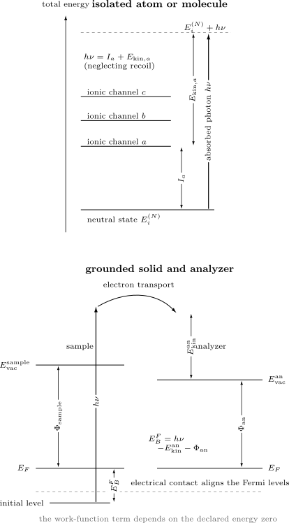
For an isolated target, a channel threshold $I_a$ and its electron kinetic energy add to $h\nu$ when recoil is neglected. For a conducting sample in electrical contact with an analyzer, Fermi levels align and the calibrated analyzer work function $\Phi_{\mathrm{an}}$ enters the usual Fermi-referenced binding-energy equation. Mixing these reference conventions creates work-function-sized errors.

Grounded conducting samples

Suppose a conducting sample and analyzer are in electrical equilibrium, so their Fermi levels align. If the analyzer reports kinetic energy relative to its own vacuum level, the conventional Fermi-referenced binding energy is

$$E_B^F = h\nu - E_{\mathrm{kin}}^{\mathrm{an}} - \Phi_{\mathrm{an}}.$$

The analyzer work function $\Phi_{\mathrm{an}}$ is part of the calibrated instrument energy scale. The sample work function does not appear as an additional subtraction in this equation: the contact potential between sample and analyzer accounts for the difference between their vacuum levels.

Relative to the sample vacuum level,

$$E_B^{\mathrm{vac}} = E_B^F+\Phi_{\mathrm{sample}}.$$

This vacuum-referenced quantity is useful for connecting a valence onset to an ionization energy, but it requires the sample work function and a clear surface condition.

Work function and secondary-electron cutoff

The sample work function is

$$\Phi_{\mathrm{sample}} = E_{\mathrm{vac}}-E_F.$$

In UPS, one can infer it from the full kinetic-energy width between the Fermi edge and secondary-electron cutoff, with the applied sample bias and analyzer convention included. A commonly used ideal relation is

$$\Phi_{\mathrm{sample}} = h\nu - \left( E_{\mathrm{Fermi}}^{\mathrm{kin}} - E_{\mathrm{cutoff}}^{\mathrm{kin}} \right).$$

The bias shifts measured kinetic energies so that low-energy electrons clear the analyzer threshold. It must be included consistently; subtracting it twice is a common failure.

Insulators, charging, and referencing

An insulating specimen may accumulate positive charge as electrons leave. A uniform electrostatic shift $\Delta V$ approximately moves all photoelectron features by

$$\Delta E_B \approx e\,\Delta V.$$

Real specimens can charge differentially, producing position-dependent shifts and broadening. A single post hoc rigid offset cannot repair a nonuniform potential distribution.

Binding-energy referencing and instrument calibration are separate tasks:

• calibration establishes the analyzer energy scale using traceable reference lines and a documented procedure;
• referencing identifies the physically relevant zero for the specimen;
• charge correction estimates specimen-induced electrostatic shifts.

Assigning an arbitrary contaminant peak a universal binding energy can hide charging, chemical shifts, or an incorrect model. Report the reference material, line, assumed value, electrical contact, neutralization method, and applied correction.

Chemical shifts are total-energy shifts

A core-level chemical shift compares channel energies in different chemical environments. It can reflect:

• initial-state charge redistribution and electrostatic potential;
• changes in screening and orbital relaxation after core-hole creation;
• multiplet and spin–orbit structure;
• local bonding, polarization, and final-state correlation;
• referencing, charging, and surface band bending.

It is therefore not a direct meter of one atomic partial charge. Interpreting a shift requires comparison within a controlled chemical series and an explicit electronic-structure or screening model.

From Ideal Channels to a Spectrum

For weak monochromatic light, a channel-resolved differential photoionization cross section has the golden-rule structure

$$\frac{d\sigma_{ai}}{d\Omega} \propto \rho_a(E_{\mathrm{kin}}) \left| M_{ai}(\mathbf k,\boldsymbol\epsilon) \right|^2.$$

The exact prefactor depends on unit system, photon-state normalization, continuum normalization, and gauge convention. A trustworthy calculation states all four. A measured spectrum then convolves this cross section with source bandwidth, target distributions, analyzer response, and electron transport.

Resolution and line shape

If statistically independent broadening contributions are approximately Gaussian, their standard deviations add in quadrature:

$$\begin{aligned} \sigma_{\mathrm{obs}}^2 &\approx \sigma_{\mathrm{photon}}^2 + \sigma_{\mathrm{analyzer}}^2 \\ &\quad+ \sigma_{\mathrm{Doppler}}^2 + \sigma_{\mathrm{other}}^2. \end{aligned}$$

The same is not true for arbitrary full widths or non-Gaussian profiles. Lorentzian lifetime widths add linearly under convolution, and a Gaussian–Lorentzian convolution gives a Voigt profile. Vibrational envelopes, unresolved multiplets, asymmetric metallic line shapes, and inelastic-loss tails require physical models rather than a larger generic width.

Line Shapes and Broadening develops these distinctions.

Analyzer acceptance and transmission

An analyzer accepts a finite energy and angular range. Its transmission $T(E,\Omega)$ can vary strongly with pass energy, lens mode, aperture, and kinetic energy. Thus an integrated band area is more accurately written

$$A_a \propto \int_{\Delta E_a}dE \int_{\Delta\Omega}d\Omega\, T(E,\Omega) \frac{d^2\sigma_a}{dE\,d\Omega}.$$

Comparing raw areas from different kinetic energies, analyzer settings, or photon energies is not a population measurement. Photoionization cross sections and asymmetry parameters also vary with photon energy.

Electron transport and surface sensitivity

In a condensed target, an electron created at depth $z$ and emitted at angle $\theta$ from the surface normal is attenuated approximately as

$$P_{\mathrm{no\ inelastic\ loss}} \sim \exp\left[ - \frac{z} {\lambda(E_{\mathrm{kin}})\cos\theta} \right],$$

where $\lambda$ is an inelastic mean free path in a simple planar model. Elastic scattering, surface roughness, anisotropy, diffraction, and finite acceptance modify this expression.

The measured signal is therefore depth weighted. Changing kinetic energy or takeoff angle changes the sampling depth. “Surface sensitive” does not mean “only the top atomic layer,” and a quoted information depth should state its criterion and transport model.

Backgrounds and energy losses

Photoelectrons that undergo inelastic scattering can populate a structured background below their original kinetic energy, equivalently at higher apparent binding energy. Plasmon losses, interband excitations, and secondary electrons are physical signals, not merely detector noise.

Background subtraction is a model choice. Shirley, Tougaard, polynomial, and locally fitted backgrounds encode different assumptions. Peak areas and satellite intensities should be reported with sensitivity to plausible background models.

Koopmans-Style Interpretation

Canonical Hartree–Fock orbitals provide a useful first assignment language. If an electron is removed from occupied spin-orbital $i$ and every remaining orbital is frozen, Koopmans’ identity gives

$$I_i^{\mathrm{frozen}} = E_{N-1}^{\mathrm{HF,frozen}}(i) - E_N^{\mathrm{HF}} = -\epsilon_i^{\mathrm{HF}}.$$

Within that constrained Hartree–Fock model, this is an exact determinant energy identity. It is not an exact statement that a measured peak equals an orbital eigenvalue.

Why it can organize a valence spectrum

For a weakly correlated closed-shell molecule:

• low-lying ionic states may be dominated by one-hole configurations;
• occupied canonical orbitals can supply symmetry and bonding labels;
• the ordering of $-\epsilon_i^{\mathrm{HF}}$ may track main-band ordering;
• Franck–Condon progressions can reveal how each ionic surface differs from the neutral surface.

This makes “ionization from orbital $i$” useful shorthand when its approximation is understood. A careful assignment says that an ionic state has dominant one-hole character associated with orbital $i$, not that the instrument measured the orbital eigenvalue directly.

Relaxation, correlation, and ionic-state mixing

After removal, the remaining electrons relax in the altered potential. Within Hartree–Fock,

$$E_{N-1}^{\mathrm{HF,opt}}(i) \le E_{N-1}^{\mathrm{HF,frozen}}(i),$$

so orbital relaxation lowers the ionized determinant energy relative to the frozen construction. Correlation changes both neutral and ionic energies and can mix several one-hole and multielectron configurations.

It is useful to audit the difference schematically:

$$\begin{aligned} I_a &= -\epsilon_i^{\mathrm{HF}} + \Delta_{\mathrm{relax},a} + \Delta_{\mathrm{corr},a} \\ &\quad+ \Delta_{\mathrm{rel},a} + \Delta_{\mathrm{nuc},a} + \cdots. \end{aligned}$$

The signs and partition of these corrections depend on definitions and method. This is an error ledger, not an independent-observable decomposition. For inner-shell holes, relaxation can be large. For open shells, removal from one determinant orbital can project onto several ionic multiplets.

Kohn–Sham eigenvalues

Kohn–Sham orbitals belong to an auxiliary system constructed to reproduce a density. Under the usual exact ground-state assumptions, the highest occupied exact Kohn–Sham eigenvalue has a special relation to the first ionization energy. This does not make every occupied eigenvalue of an approximate functional an exact photoelectron binding energy.

Generalized Kohn–Sham eigenvalues can be useful empirical assignment tools, but comparisons must state the functional, orbital convention, geometry, relativistic treatment, and whether energies were obtained from orbital eigenvalues, total-energy differences, quasiparticle theory, or an explicit ionized-state calculation.

A practical hierarchy

For peak positions, increasingly complete models include:

1. frozen-orbital Hartree–Fock estimates;
2. separately optimized neutral and ionic total-energy differences;
3. correlated ionization-potential or electron-propagator methods;
4. vibronic, relativistic, and continuum-coupled calculations;
5. explicit simulation of instrumental and transport response.

Higher on this list does not automatically mean better. A calculation must converge the relevant states, represent the continuum, and match the measured observable. A highly correlated bound-state energy with a crude continuum can predict peak positions well while failing angular distributions.

Molecular-Orbital Information

A photoelectron spectrum contains genuine orbital information, but only through state-to-state removal amplitudes and a forward model.

Dyson orbitals

For normalized initial state $\Psi_i^{(N)}$ and ionic state $\Psi_a^{(N-1)}$, define the Dyson spin-orbital

$$\begin{aligned} \phi_{D,ai}(x) &= \sqrt N \int dX\, \Psi_a^{(N-1)*}(X) \\ &\quad\times \Psi_i^{(N)}(x,X). \end{aligned}$$

It is the overlap left after $N-1$ electron coordinates have been integrated out. Different ionic states have different Dyson orbitals, even when a one-orbital picture assigns them to the same nominal shell.

In a single-channel, sudden, dipole description, the amplitude can often be organized as

$$M_{ai}(\mathbf k,\boldsymbol\epsilon) \approx \left\langle \chi_{\mathbf k,a}^{(-)} \middle| \boldsymbol\epsilon\cdot\widehat{\mathbf d} \middle| \phi_{D,ai} \right\rangle,$$

where $\chi_{\mathbf k,a}^{(-)}$ is a continuum electron state distorted by the ionic channel. This compact expression is powerful, but it is an approximation to a fully antisymmetrized many-electron scattering amplitude. Interchannel coupling and correlation in the continuum may not factorize.

Pole strength and one-electron character

The Dyson-orbital norm

$$Z_{ai} = \int dx\, \left| \phi_{D,ai}(x) \right|^2$$

is often called a pole strength or spectroscopic factor in an appropriate Green-function convention. A value near one indicates strong one-electron removal character for that channel. Correlation can distribute strength across many ionic states so that individual $Z_{ai}$ values are smaller.

Measured integrated intensity is not generally equal to $Z_{ai}$:

$$A_a \not\propto Z_{ai} \quad\text{without further assumptions}.$$

It also contains continuum matrix elements, photon-energy dependence, polarization, molecular orientation, degeneracy, analyzer acceptance, and transport. Pole strength is a property of the many-body overlap; observed area is a property of the full experiment.

Main lines and satellites

In a one-hole picture, a main line connects strongly to an ionic state dominated by deleting one occupied orbital. Correlation can create additional channels:

• shake-up: ionization accompanied by a bound excitation of the residual system;
• shake-off: ionization accompanied by emission of another electron into the continuum;
• multiplet splitting: several ionic terms formed by coupling the hole to open-shell angular momenta;
• screened and unscreened final states: distinct many-body responses to a hole, especially in solids and transition-metal compounds;
• plasmon or other loss structures: extrinsic, intrinsic, or interfering energy-loss processes.

A weak satellite need not be contamination, and a strong satellite need not represent a highly occupied orbital. Satellite positions and intensities are among the most direct signs that the one-hole approximation is incomplete.

Cross-section zeros and missing bands

Even a channel with substantial Dyson norm can become weak if its dipole matrix element is small. A radial dipole integral can pass through zero as photon energy varies, producing a Cooper minimum in a partial photoionization cross section. Symmetry, orientation averaging, destructive partial-wave interference, and detector geometry can likewise suppress a band.

Absence from one spectrum is therefore not proof that an orbital or ionic state does not exist. Varying photon energy and polarization is a central assignment test.

Extended systems and spectral functions

For a translationally ordered solid, angle-resolved photoemission can be related under a sudden, single-particle-like treatment to

$$I(\mathbf k,\omega) \propto \left| M(\mathbf k,\omega) \right|^2 f(\omega) A(\mathbf k,\omega),$$

convolved with resolution and supplemented by background and surface effects. Here $A(\mathbf k,\omega)$ is the electron-removal spectral function and $f$ is the occupation factor.

This formula is a useful map, not a license to identify intensity directly with $A$. Matrix-element zeros, finite escape depth, surface states, $k_z$ uncertainty, final-state structure, domains, and detector acceptance all matter. Spectral Functions owns the Lehmann representation, quasiparticle poles, and incoherent weight.

Photoelectron Angular Distributions

Energy conservation says which channel is open. The angular distribution reveals how photon polarization, target symmetry, continuum angular momenta, and scattering phases combine within that channel.

Random targets and linearly polarized light

For one-photon ionization of a randomly oriented target in the electric-dipole approximation, with no resolved electron spin, the laboratory-frame distribution has the form

$$\frac{d\sigma}{d\Omega} = \frac{\sigma_{\mathrm{tot}}}{4\pi} \left[ 1+\beta P_2(\cos\theta) \right],$$

where

$$P_2(\cos\theta) = \frac{1}{2} \left( 3\cos^2\theta-1 \right).$$

The angle $\theta$ is measured from the linear-polarization axis. Positivity imposes

$$-1\le\beta\le2.$$

Three limiting patterns are useful:

$\beta$	Angular character	Relative pattern
$2$	Strongly parallel	$\cos^2\theta$
$0$	Isotropic in this laboratory frame	constant
$-1$	Strongly perpendicular	$\sin^2\theta$

Because

$$\int d\Omega\,P_2(\cos\theta)=0,$$

the distribution integrates to $\sigma_{\mathrm{tot}}$. An analyzer at one angle samples a $\beta$-dependent fraction of the total cross section.

At the magic angle

$$\begin{gathered} P_2(\cos\theta_m)=0, \\ \theta_m = \arccos\left(\frac{1}{\sqrt3}\right), \\ \theta_m\approx54.7^\circ. \end{gathered}$$

the dipole anisotropy term vanishes. This can simplify comparisons, but only when the target, polarization, acceptance, and dipole assumptions fit the formula.

Partial waves and dipole selection

For an atomic electron with initial orbital angular momentum $\ell$, an electric-dipole transition produces continuum channels

$$\ell' = \ell\pm1.$$

Their radial amplitudes and scattering phases interfere. The total cross section depends on squared amplitudes, while $\beta$ also depends on relative phases. Thus two models can predict similar total yield but different angular patterns.

A Cooper minimum occurs when a relevant radial dipole matrix element changes sign through zero. Near the minimum:

• the partial cross section can become small;
• a normally subdominant channel can control the angular pattern;
• $\beta$ can vary rapidly;
• correlation and relativistic channel coupling become conspicuous.

This is scattering-phase information encoded in photoemission.

Molecules and molecular-frame distributions

For a randomly oriented molecule, orientation averaging reduces a one-photon dipole distribution to the same $1+\beta P_2$ form. That single number does not retain the complete molecular-frame pattern.

If the molecular axis is known through alignment, orientation, or coincident fragment recoil, the differential cross section can depend on several angles and polarization tensors. Molecular-frame photoelectron angular distributions can expose nodal structure, shape resonances, multicenter interference, and the symmetry of the residual ion.

Reconstructing an “orbital image” from such data requires:

• a state-specific ionic channel;
• a continuum scattering model;
• an orientation and recoil model;
• a gauge and phase convention;
• treatment of finite resolution and detector acceptance.

The reconstructed object is a model-dependent transition amplitude, often closely related to a Dyson orbital, not a photograph of a stationary electron cloud.

Beyond the simple anisotropy formula

Additional angular coefficients are required for:

• oriented or aligned targets;
• circular or elliptical polarization;
• spin-resolved detection;
• nondipole electric-quadrupole and magnetic-dipole contributions;
• multiphoton ionization;
• chiral photoelectron circular dichroism;
• coincident electrons or fragments.

At higher photon energies, terms odd in the photon propagation direction can produce forward–backward asymmetry. Fitting such data with only $\beta$ can fold nondipole physics into a misleading dipole parameter.

Thresholds, Resonances, and Scattering

The emitted electron is a scattering particle in the field of the residual target. Photoionization is therefore a bound-to-continuum scattering problem, not merely a bound-state energy difference.

Wigner threshold law

For a short-range residual interaction and an outgoing partial wave $\ell$, the near-threshold partial cross section behaves as

$$\sigma_\ell \propto k^{2\ell+1},$$

or, since $E_{\mathrm{kin}}\propto k^2$,

$$\sigma_\ell \propto E_{\mathrm{kin}}^{\ell+1/2}.$$

The lowest allowed partial wave usually dominates sufficiently close to threshold. For photodetachment into an $s$ wave, $\sigma\propto E_{\mathrm{kin}}^{1/2}$; for a $p$ wave, $\sigma\propto E_{\mathrm{kin}}^{3/2}$.

The assumptions matter. A residual positive ion has an attractive Coulomb tail, for which the simple short-range exponent is modified. Polarization potentials, dipole-bound states, virtual states, resonances, and channel coupling can also alter the observed onset.

Direct ionization and autoionization

In direct photoionization, the photon couples directly to an open ion-plus-electron channel. A photon can also excite a discrete state embedded in a continuum, which then decays by ejecting an electron. Interference between direct and resonant paths can produce a Fano profile:

$$\sigma(\epsilon) \propto \frac{(q+\epsilon)^2}{1+\epsilon^2}, \qquad \epsilon = \frac{2(E-E_r)}{\Gamma}.$$

Here $E_r$ and $\Gamma$ locate and broaden the resonance, while $q$ encodes the relative resonant and direct amplitudes in the ideal one-continuum model. The asymmetric profile is amplitude interference, not two unresolved positive peaks.

Autoionization and Auger decay are related but distinct labels. In autoionization, an excited state above an ionization threshold ejects an electron through electron correlation. In an Auger process, a vacancy is filled while another electron is emitted. The latter electron kinetic energy is primarily set by electronic level differences and is not shifted one for one with the exciting photon energy.

Continuum boundary conditions

The state $\chi_{\mathbf k}^{(-)}$ in a photoionization matrix element carries incoming-wave scattering boundary conditions in a common bra convention; its complex conjugate represents the physically outgoing electron. Other conventions use a $(+)$ state in the ket. Either is valid if phases, normalization, and matrix elements are handled consistently.

The partial-wave form is schematically

$$\begin{aligned} \chi_{\mathbf k}^{(-)}(\mathbf r) &= \sum_{\ell m} C_{\ell m}(\widehat{\mathbf k})\, e^{-i\delta_\ell(E)} \\ &\quad\times R_{\ell E}(r) Y_{\ell m}(\widehat{\mathbf r}). \end{aligned}$$

The scattering phase shifts $\delta_\ell(E)$ control angular interference and resonance behavior. A plane-wave final state discards these phases and can fail badly at low energy, near shape resonances, around Cooper minima, or in multicenter molecular potentials.

Time-reversed photorecombination

Microscopic reversibility relates state-resolved photoionization to the time-reversed radiative recombination process,

$$\mathrm{A} + h\nu \rightleftharpoons \mathrm{A}^+ + e^-.$$

Detailed-balance factors account for phase-space and degeneracy differences. The same dipole amplitudes and continuum phases appear in both directions. High-harmonic recombination also probes a related time-reversed matrix element, although strong-field preparation and propagation add substantial physics.

Scattering inside the target

For molecules and solids, the outgoing wave can scatter from neighboring centers before detection. This produces:

• molecular shape resonances;
• multicenter interference;
• photoelectron diffraction;
• energy-dependent final-state phases;
• elastic deflection and inelastic losses.

The relation to scattering is therefore twofold: scattering theory defines the final continuum state, and actual post-emission transport reshapes the detected distribution.

Reading Atomic, Molecular, and Solid Spectra

The same conservation law produces different diagnostic structures in different targets.

Atoms

Atomic spectra can show:

• subshell thresholds and spin–orbit doublets;
• ionic term and multiplet splitting;
• Cooper minima and autoionizing resonances;
• angular-distribution and spin-polarization structure;
• correlation satellites and double-ionization continua.

A subshell label such as $3p$ does not specify one line when spin–orbit, open-shell coupling, and multiple ionic terms are resolved.

Molecules

Molecular spectra can show:

• bands associated with distinct ionic electronic states;
• vibrational progressions and geometry change;
• Jahn–Teller or Renner–Teller structure in degenerate states;
• conformer, tautomer, and temperature dependence;
• dissociative ionization and channel-specific fragmentation;
• shape resonances and molecular-frame angular patterns.

Band assignment should combine energy, vibrational structure, symmetry, isotopic substitution, photon-energy dependence, angular distributions, and electronic-structure calculations. Matching one vertical ionization energy is not enough.

Solids and surfaces

Solid-state photoemission can show:

• a Fermi edge and occupied valence bands;
• core-level chemical shifts and spin–orbit components;
• surface and bulk components;
• quasiparticle peaks and incoherent satellites;
• plasmons and other energy-loss structures;
• band bending, charging, and contact-potential effects;
• momentum-dependent dispersion in ARPES.

Core-level area ratios require sensitivity factors that include subshell cross sections, analyzer transmission, angular asymmetry, attenuation, and sample geometry. Nominal degeneracy alone is not a universal intensity calibration.

A Measurement and Assignment Workflow

1. Define the question

State whether the target observable is:

• an adiabatic or vertical gas-phase ionization energy;
• an ionic-state vibrational spacing;
• a core-level chemical shift;
• elemental composition or depth profile;
• a total or differential cross section;
• an angular anisotropy;
• a band dispersion or spectral-function feature.

Different observables require different calibrations and theory.

2. Declare source and target conditions

Record photon energy, bandwidth, polarization, incidence geometry, flux, and harmonic contamination. Record target temperature, pressure, composition, phase, substrate, preparation, electrical contact, bias, and radiation dose.

For molecules, identify conformers, clusters, hot bands, and carrier gas. For solids, identify surface cleanliness, crystallographic orientation, charging, neutralization, and beam-induced change.

3. Calibrate the analyzer

Document:

• reference lines and accepted energies;
• pass energy and lens mode;
• linearity and drift checks across the energy range;
• analyzer work-function or software energy convention;
• estimated calibration uncertainty.

Calibration at one energy does not prove linearity over hundreds of electronvolts.

4. Separate calibration from sample referencing

For a conducting solid, verify Fermi-level contact. For an insulator, test flux, neutralizer, thickness, substrate, and spatial dependence. Report every rigid shift applied to the spectrum and its rationale.

For isolated species, calibrate photon and electron energies independently where possible and include recoil or contact-potential corrections at the claimed precision.

5. Measure resolution and response

Determine source bandwidth, analyzer response, angular acceptance, and transmission under the actual settings. Do not infer physical linewidths below the calibrated instrumental width without deconvolution and uncertainty analysis.

6. Build an energy-first channel table

For each candidate feature, tabulate:

Quantity	Evidence
Measured position and uncertainty	Calibrated spectrum and fit
Proposed residual state	Symmetry, term, vibrational state, or band
Predicted total-energy difference	Declared electronic-structure model
Expected splitting or progression	Spin–orbit, multiplet, or vibrational model
Photon-energy and polarization trend	Cross-section and angular-distribution model
Alternative assignment	Contaminant, loss, satellite, charging, or another channel

This prevents a visually attractive orbital diagram from becoming the entire argument.

7. Stress-test intensities

Repeat or model the measurement at more than one photon energy or polarization when feasible. Correct for analyzer transmission and attenuation. Vary background and line-shape models. Check whether a weak feature tracks a main line like an energy-loss satellite or follows its own threshold and angular behavior.

8. Report uncertainty at the inference level

Separate:

• statistical peak-position and area uncertainty;
• calibration and referencing uncertainty;
• line-shape and background-model uncertainty;
• sample heterogeneity and charging;
• theoretical truncation, basis, geometry, and relativistic uncertainty;
• ambiguity among assignments.

Numerical agreement smaller than the combined uncertainty is not evidence that one orbital interpretation is uniquely correct.

Common Mistakes

“A peak is the energy of an electron in an orbital”

A peak is a transition energy between an $N$-electron initial state and a specific $(N-1)$-electron final channel, plus declared nuclear and reference conventions. Orbital eigenvalues can approximate or organize these differences.

“Peak area counts electrons”

Area also depends on cross section, photon energy, polarization, continuum dynamics, degeneracy, analyzer transmission, attenuation, and background. Electron counting requires a calibrated model.

“The tallest valence peak is the HOMO”

The lowest-binding-energy threshold is associated with the first accessible ionization channel. Its peak may be weak, unresolved, symmetry suppressed, or thermally broadened. Height is not an energy-ordering criterion.

“Vertical ionization energy is the band maximum”

The vertical energy is a fixed-geometry total-energy difference. The band maximum emerges from a vibronic envelope multiplied by energy-dependent matrix elements and convolved with resolution.

“Koopmans’ theorem predicts the experimental spectrum”

It predicts frozen-orbital Hartree–Fock determinant differences. Relaxation, correlation, ionic-state mixing, nuclear motion, relativity, and continuum matrix elements remain.

“Every weak extra line is an impurity”

Satellites, hot bands, isotopologues, multiplets, loss structures, and autoionizing channels can be intrinsic. Impurity assignment requires controlled composition and correlated spectral evidence.

“All XPS binding energies use the sample work function”

For a grounded conductor measured by a calibrated analyzer, the standard Fermi-referenced equation uses the analyzer work function. Vacuum-referenced energies and insulating samples require additional information.

“A rigid charge correction always fixes an insulating spectrum”

It works only for an effectively uniform potential shift. Differential charging changes separations and widths and cannot be repaired by one offset.

“The anisotropy parameter is an orbital shape”

$\beta$ is a channel- and energy-dependent interference observable. It depends on continuum amplitudes and phases as well as the initial-state symmetry.

“A plane wave is always adequate at high kinetic energy”

High energy can improve a plane-wave approximation, but atomic and molecular scattering, diffraction, nondipole effects, surface potentials, and matrix-element zeros can remain decisive. Adequacy is an observable-specific convergence question.

Worked Examples

Gas-phase channel assignment

A He I source supplies

$$h\nu=21.218\ \mathrm{eV}.$$

A molecular band has calibrated electron kinetic energy

$$E_{\mathrm{kin}}=11.750\ \mathrm{eV}.$$

Neglecting recoil at the quoted precision gives

$$\begin{aligned} I &= h\nu-E_{\mathrm{kin}} \\ &= 21.218\ \mathrm{eV} - 11.750\ \mathrm{eV} \\ &= 9.468\ \mathrm{eV}. \end{aligned}$$

This number labels the populated ionic channel. Calling it a HOMO energy requires the additional claim that the channel is dominated by removal from the neutral HOMO and that a Koopmans-like interpretation is adequate.

Analyzer-referenced XPS

For monochromated Al $K\alpha$ radiation, take

$$h\nu=1486.70\ \mathrm{eV}.$$

If the analyzer reports $E_{\mathrm{kin}}^{\mathrm{an}}=1200.00\ \mathrm{eV}$ and its calibrated work function is $\Phi_{\mathrm{an}}=4.20\ \mathrm{eV}$, then

$$\begin{aligned} E_B^F &= h\nu - E_{\mathrm{kin}}^{\mathrm{an}} - \Phi_{\mathrm{an}} \\ &= 282.50\ \mathrm{eV}. \end{aligned}$$

Subtracting the sample work function again would double count the contact potential convention.

Angular acceptance

For $\beta=1.5$, the ideal differential intensity along the polarization axis is proportional to

$$1+\beta=2.5.$$

At $90^\circ$,

$$1-\frac{\beta}{2}=0.25.$$

An infinitesimal detector parallel to the polarization therefore sees ten times the differential intensity of one at $90^\circ$:

$$\frac{I(0^\circ)}{I(90^\circ)} = \frac{2.5}{0.25} = 10.$$

A real analyzer averages over finite angular acceptance, so its measured ratio is less extreme unless the acceptance integration is included.

Exercises

Exercise 1: Recoil audit

A photon of energy $40.000\ \mathrm{eV}$ ionizes a stationary molecule into a channel with threshold $12.300\ \mathrm{eV}$. The measured electron kinetic energy is $27.699\ \mathrm{eV}$. Assuming no fragmentation, what recoil energy is implied? Would it be consistent to quote the threshold to $0.1\ \mathrm{meV}$ while neglecting this term?

Solution

Energy conservation gives

$$E_{\mathrm{recoil}} = h\nu-I-E_{\mathrm{kin}}.$$

Therefore

$$\begin{aligned} E_{\mathrm{recoil}} &= 40.000\ \mathrm{eV} - 12.300\ \mathrm{eV} \\ &\quad- 27.699\ \mathrm{eV} \\ &= 0.001\ \mathrm{eV} = 1\ \mathrm{meV}. \end{aligned}$$

The recoil correction is ten times the proposed $0.1\ \mathrm{meV}$ precision. It cannot be neglected at that level. One must also audit photon energy, thermal motion, and calibration uncertainties before claiming such a threshold.

Exercise 2: Vertical versus adiabatic ionization

At the neutral equilibrium geometry, a calculation gives a vertical ionization energy of $9.80\ \mathrm{eV}$. Relaxing the ion lowers its electronic energy by $0.34\ \mathrm{eV}$ relative to that vertical ionic geometry. The ionic zero-point energy exceeds the neutral zero-point energy by $0.05\ \mathrm{eV}$. Estimate the adiabatic ionization energy. Why need neither value coincide exactly with the band maximum?

Solution

The relaxed electronic minimum lowers the ionization difference by $0.34\ \mathrm{eV}$, while the zero-point difference raises it by $0.05\ \mathrm{eV}$:

$$\begin{aligned} I^{\mathrm{ad}} &= 9.80\ \mathrm{eV} - 0.34\ \mathrm{eV} + 0.05\ \mathrm{eV} \\ &= 9.51\ \mathrm{eV}. \end{aligned}$$

The adiabatic energy refers to the two lowest rovibronic levels under the stated model. The vertical energy is a fixed-geometry difference. A measured band maximum is selected by the Franck–Condon envelope, rotational and thermal populations, matrix-element variation, linewidths, and instrument response, so it is not defined by either energy alone.

Exercise 3: Work-function conventions

A grounded conducting sample is measured with photons of $h\nu=1486.70\ \mathrm{eV}$. The analyzer work function is $4.30\ \mathrm{eV}$ and the measured kinetic energy is $1200.10\ \mathrm{eV}$. The independently measured sample work function is $5.10\ \mathrm{eV}$.

1. Find the Fermi-referenced binding energy.
2. Find the sample-vacuum-referenced binding energy.
3. Explain why the sample work function is absent from the first calculation.

Solution

The Fermi-referenced value is

$$\begin{aligned} E_B^F &= h\nu - E_{\mathrm{kin}}^{\mathrm{an}} - \Phi_{\mathrm{an}} \\ &= 1486.70 - 1200.10 - 4.30 \\ &= 282.30\ \mathrm{eV}. \end{aligned}$$

The vacuum-referenced value is

$$\begin{aligned} E_B^{\mathrm{vac}} &= E_B^F+\Phi_{\mathrm{sample}} \\ &= 287.40\ \mathrm{eV}. \end{aligned}$$

Electrical contact aligns sample and analyzer Fermi levels. Their unequal work functions create a contact potential that shifts the electron kinetic energy en route to the analyzer. Using the analyzer-referenced kinetic energy and calibrated analyzer work function already includes that shift.

Exercise 4: Koopmans and relaxation

An occupied Hartree–Fock orbital has $\epsilon_i=-15.0\ \mathrm{eV}$. Reoptimizing the ionic Hartree–Fock determinant lowers its energy by $2.2\ \mathrm{eV}$ relative to the frozen ion. Correlation and relativistic corrections together raise the predicted ionization energy by $0.7\ \mathrm{eV}$ relative to the relaxed Hartree–Fock value. Estimate the three successive ionization energies and identify which one Koopmans’ theorem supplies.

Solution

Koopmans’ frozen-orbital value is

$$I_i^{\mathrm{frozen}} = -\epsilon_i = 15.0\ \mathrm{eV}.$$

Relaxation lowers the ionic total energy and hence the ionization energy:

$$I_i^{\mathrm{relaxed\ HF}} = 15.0-2.2 = 12.8\ \mathrm{eV}.$$

The stated remaining corrections raise it:

$$I_i^{\mathrm{corrected}} = 12.8+0.7 = 13.5\ \mathrm{eV}.$$

Only the first value is the frozen-orbital Koopmans result. The numerical partition is model dependent; in a real calculation, correlation corrections must be computed for both neutral and ionic states rather than added by rule of thumb.

Exercise 5: Pole strength is not peak area

Two ionic channels have Dyson norms $Z_1=0.80$ and $Z_2=0.40$. At one photon energy, the continuum and detector factors multiplying these norms are in the ratio $C_1:C_2=1:3$. Under the simplified model $A_a\propto C_aZ_a$, what area ratio is expected? What lesson survives when the factorization itself fails?

Solution

The simplified areas satisfy

$$\frac{A_1}{A_2} = \frac{C_1Z_1}{C_2Z_2} = \frac{1\times0.80}{3\times0.40} = \frac{2}{3}.$$

The channel with the larger Dyson norm has the smaller observed area because its continuum and detection factor is weaker. More generally, the exact amplitude may not factor into a pole strength times a scalar continuum factor. The robust lesson is that a peak area is not a direct measurement of Dyson norm, occupancy, or electron count.

Exercise 6: Normalize an angular distribution

Show that

$$\frac{d\sigma}{d\Omega} = \frac{\sigma}{4\pi} \left[ 1+\beta P_2(\cos\theta) \right]$$

integrates to $\sigma$. Then find the parallel-to-perpendicular differential intensity ratio for $\beta=1.2$.

Solution

Using $d\Omega=2\pi\,d(\cos\theta)$ and

$$\int_{-1}^{1}P_2(u)\,du=0,$$

one obtains

$$\begin{aligned} \int d\Omega\, \frac{d\sigma}{d\Omega} &= \frac{\sigma}{4\pi} \left[ 4\pi + \beta(0) \right] \\ &= \sigma. \end{aligned}$$

At $0^\circ$, the angular factor is $1+\beta=2.2$. At $90^\circ$, $P_2(0)=-1/2$, so it is $1-\beta/2=0.4$. Hence

$$\frac{I(0^\circ)}{I(90^\circ)} = \frac{2.2}{0.4} = 5.5.$$

Exercise 7: Threshold exponents

For a short-range residual potential, compare the increase in cross section when the excess energy rises from $E$ to $4E$ for an outgoing $s$ wave and for an outgoing $p$ wave.

Solution

Wigner’s law gives

$$\sigma_\ell \propto E^{\ell+1/2}.$$

For an $s$ wave, $\ell=0$:

$$\frac{\sigma_s(4E)}{\sigma_s(E)} = 4^{1/2} = 2.$$

For a $p$ wave, $\ell=1$:

$$\frac{\sigma_p(4E)}{\sigma_p(E)} = 4^{3/2} = 8.$$

The lower allowed partial wave rises more slowly but dominates sufficiently close to threshold because higher partial waves are more strongly suppressed. The result must not be applied unchanged to an attractive Coulomb residual potential.

Exercise 8: Diagnose an unexpected XPS feature

An insulating oxide shows a new weak peak on the high-binding-energy side of a main core line. Its separation from the main line is constant as photon flux changes, but both features broaden and shift nonrigidly across the illuminated spot. List the tests needed before assigning the feature as a shake-up satellite.

Solution

The constant separation is compatible with an intrinsic satellite, but the nonrigid spatial and flux-dependent shifts diagnose differential charging. Before assignment:

• vary photon flux, dwell time, neutralizer settings, and electrical contact;
• map position across the spot and compare conductive or thinner specimens;
• verify analyzer calibration independently of charge referencing;
• test several physically plausible backgrounds and line shapes;
• vary photon energy to change cross sections and escape depths;
• compare the feature’s intensity and width with the main line;
• inspect related core levels and expected energy-loss structures;
• compare with a many-electron final-state calculation or controlled chemical reference;
• check beam damage, contamination, phase mixtures, and sample history.

An intrinsic shake-up assignment becomes credible only if the feature survives charging controls and follows the expected chemical, photon-energy, and many-body trends.

Further Connections

• Spectroscopy Overview supplies the source–target–evolution–detector measurement chain.
• Ultrafast Spectroscopy Overview explains how delayed ionization gates evolving electronic and nuclear wave packets.
• Transition Rates develops golden-rule rates and densities of continuum states.
• Selection Rules in Spectroscopy distinguishes exact zeros from approximate and geometry-dependent propensities.
• Line Shapes and Broadening develops lifetime, dephasing, inhomogeneous, Doppler, and instrumental broadening.
• Molecular Orbitals owns the LCAO, symmetry, occupation, and Koopmans language used in valence assignments.
• Electronic Structure Overview compares total-energy, ionized-state, propagator, and multireference methods.
• Born–Oppenheimer in Molecules provides the electronic potential surfaces underlying vertical and adiabatic ionization.
• Atomic Orbitals Revisited gives the canonical interpretation of Hartree–Fock, Kohn–Sham, natural, localized, and Dyson orbitals.
• Hartree–Fock for Atoms derives the frozen-orbital Koopmans identity and orbital-relaxation inequality.
• Spectral Functions develops the many-body removal spectrum, quasiparticle residue, and incoherent weight.
• Edge and Surface States applies angle-resolved and spin-resolved photoemission to surface Dirac cones, Fermi arcs, matrix-element caveats, and bulk-versus-surface tests.
• Partial-Wave Expansion and Phase Shifts develop the continuum machinery behind angular distributions.
• Cross Sections distinguishes total, differential, and acceptance-integrated observables.
• Coulomb Continuum States Overview explains why an ionic Coulomb tail changes free-wave and threshold intuition.

References

• IUPAC, “photoelectron spectroscopy,” Compendium of Chemical Terminology, 5th ed. — measurement definition and PES, UPS, XPS, and ESCA terminology.
• IUPAC, “ionization energy,” Compendium of Chemical Terminology — adiabatic and vertical ionization-energy terminology.
• T. Koopmans, “Über die Zuordnung von Wellenfunktionen und Eigenwerten zu den einzelnen Elektronen eines Atoms,” Physica 1, 104–113 (1934), doi:10.1016/S0031-8914(34)90011-2 — original frozen-orbital relation.
• J. Cooper and R. N. Zare, “Angular Distribution of Photoelectrons,” Journal of Chemical Physics 48, 942–943 (1968), doi:10.1063/1.1668742 — dipole anisotropy formula and partial-wave interpretation.
• E. P. Wigner, “On the Behavior of Cross Sections Near Thresholds,” Physical Review 73, 1002–1009 (1948), doi:10.1103/PhysRev.73.1002 — threshold laws and the role of long-range product interactions.
• U. Fano, “Effects of Configuration Interaction on Intensities and Phase Shifts,” Physical Review 124, 1866–1878 (1961), doi:10.1103/PhysRev.124.1866 — interference between discrete and continuum pathways.
• J. J. Yeh and I. Lindau, “Atomic Subshell Photoionization Cross Sections and Asymmetry Parameters: $1\le Z\le103$,” Atomic Data and Nuclear Data Tables 32, 1–155 (1985), doi:10.1016/0092-640X(85)90016-6 — tabulated photon-energy-dependent cross sections and anisotropies.
• NIST Standard Reference Database 20, X-ray Photoelectron Spectroscopy Database, version 4.1 — evaluated binding energies, chemical shifts, Auger energies, and measurement metadata.
• C. J. Powell, “Calibrations and Checks of the Binding-Energy Scales of X-ray Photoelectron Spectrometers,” Journal of Electron Spectroscopy and Related Phenomena 257, 146808 (2022), doi:10.1016/j.elspec.2018.11.007 — analyzer calibration, reference energies, drift, and uncertainty.
• M. P. Seah, I. S. Gilmore, and S. J. Spencer, “Measurement of Data for and the Development of an ISO Standard for the Energy Calibration of X-ray Photoelectron Spectrometers,” Surface and Interface Analysis 31, 778–795 (2001), doi:10.1002/sia.1115 — multi-line binding-energy calibration procedure.
• C. S. Fadley, “X-ray Photoelectron Spectroscopy: Progress and Perspectives,” Journal of Electron Spectroscopy and Related Phenomena 178–179, 2–32 (2010), doi:10.1016/j.elspec.2010.01.006 — core-level photoemission, diffraction, surfaces, and modern extensions.
• J. W. Rabalais, Principles of Ultraviolet Photoelectron Spectroscopy, Wiley, 1977 — molecular valence ionization, vibronic structure, and angular distributions.
• D. W. Turner, C. Baker, A. D. Baker, and C. R. Brundle, Molecular Photoelectron Spectroscopy, Wiley-Interscience, 1970 — foundational gas-phase molecular photoelectron spectroscopy.
• S. Hüfner, Photoelectron Spectroscopy: Principles and Applications, 3rd ed., Springer, 2003, doi:10.1007/978-3-662-09280-4 — photoemission from atoms, molecules, solids, and surfaces.
• C. M. Truesdale, S. Southworth, P. H. Kobrin, U. Becker, D. W. Lindle, H. G. Kerkhoff, and D. A. Shirley, “Photoelectron Angular Distributions of Molecular Nitrogen in the Shape-Resonance Region,” Physical Review Letters 50, 1265–1269 (1983), doi:10.1103/PhysRevLett.50.1265 — continuum scattering and molecular shape-resonance anisotropy.
• A. Müller et al., “Time-Reversal Studies in Photorecombination and Photoionization Experiments with Ion Beams,” AIP Conference Proceedings 680, 1–10 (2003), doi:10.1063/1.1619696 — state-resolved detailed balance between photoionization and photorecombination.

Frontier Context

Attosecond and Ultrafast Frontiers tracks dated evidence and open questions in photoemission timing, ion–photoelectron entanglement, attosecond streaking, RABBITT interferometry, and strong-field ionization. The binding-energy conventions, channel amplitudes, angular distributions, threshold laws, and continuum-scattering foundations developed here remain canonical.