Electronic Structure Methods Map
An electronic-structure method is defensible only relative to a declared claim. “Use DFT,” “use coupled cluster,” or “use a multireference method” does not yet specify a calculation. One must also state the electronic state, property, geometry, Hamiltonian, nuclear model, one-particle representation, method variant, numerical solver, convergence thresholds, and validation evidence.
The practical question is therefore not
Which acronym is best?
but
Which controlled approximation can answer this particular question, at this geometry and accuracy target, and what evidence would reveal its failure?
This page turns that question into a workflow. It compares Hartree–Fock (HF), density-functional theory (DFT), configuration interaction (CI), coupled cluster (CC), multireference methods, quantum Monte Carlo (QMC), and time-dependent or response methods. The comparison is deliberately conditional. None of these families is uniformly more accurate than all the others across ground states, excited states, bond breaking, weak interactions, transition metals, heavy elements, and extended systems.
Canonical Scope
Section titled “Canonical Scope”Electronic Structure Overview owns the formal introductions to the electronic Hamiltonian, orbital bases, HF, CI, CC, DFT, CASSCF, and excited-state expansions. Hartree–Fock Approximation owns the determinant variational derivation. Atomic Correlation Methods Overview owns the atomic-structure implementation perspective. Quantum Monte Carlo Preview and Variational Monte Carlo Preview own broader stochastic-many-body foundations.
This page owns the operational methods map:
- how to define the target before selecting a method;
- which assumptions distinguish the main method families;
- where each family commonly succeeds or fails;
- how formal cost estimates should and should not be used;
- which diagnostics deserve attention;
- how to design method–basis convergence studies;
- how to separate solver, representation, method, and physical-model error;
- how to validate a calculation without tuning it to one desired answer;
- and which metadata makes a method choice reproducible.
Brief equations identify each family, but full derivations remain at their canonical homes.
A Calculation Is More Than a Method Name
Section titled “A Calculation Is More Than a Method Name”A useful abstraction is a calculation specification
Its entries are:
| Symbol | Meaning | Example |
|---|---|---|
| Hamiltonian and external fields | nonrelativistic clamped-nuclei Coulomb Hamiltonian | |
| nuclear and environmental model | fixed nuclei, continuum solvent, or periodic cell | |
| state sector | charge, spin, spatial symmetry, and targeted root | |
| one-particle representation | Gaussian basis, plane waves, grid, or numerical orbitals | |
| electronic ansatz or functional | CCSD(T), a named density functional, or CASSCF active space | |
| solver and algorithmic choices | SCF optimizer, eigensolver, walker algorithm, or propagator | |
| numerical thresholds | integral, energy, residual, grid, and statistical tolerances | |
| property protocol | analytic derivative, response theory, finite field, or energy difference |
The reported quantity is then more honestly written as
or, for density-based methods,
Two results with the same method label but different Hamiltonians, basis sets, spin constraints, geometries, grids, or property definitions need not be comparable.
Model chemistry
Section titled “Model chemistry”In practical quantum chemistry, a declared method together with its basis, Hamiltonian, and auxiliary approximations is often called a model chemistry. A model chemistry should behave as a transferable protocol, not as a menu from which options are silently changed until one datum agrees with experiment.
For an energy difference,
the same protocol should normally be applied to both states and . Balanced error is usually more important than either absolute total energy considered alone.
Claim first, calculation second
Section titled “Claim first, calculation second”The following claims are different computational problems:
- the equilibrium bond length of one electronic state;
- a vertical electronic excitation at a fixed geometry;
- an adiabatic excitation including relaxation;
- a dissociation energy including zero-point motion;
- a spin-state energy gap;
- an intermolecular binding energy;
- a transition dipole or oscillator strength;
- a nonadiabatic derivative coupling;
- a core-level ionization energy;
- or a real-time response to a strong pulse.
The method, basis, state tracking, relativistic model, and validation target can change when the claim changes.
Decision Workflow
Section titled “Decision Workflow”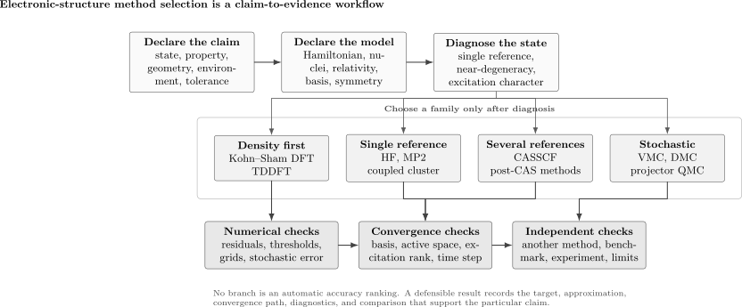
Method selection begins with the claim and Hamiltonian, not with an accuracy ranking. State diagnosis narrows plausible method families; numerical, convergence, and independent checks then determine whether the resulting claim is supported.
A practical first pass is:
- Name the observable and state. Include charge, spin, symmetry, root, geometry, and whether the target is vertical, adiabatic, or dynamical.
- Choose the physical model. State the Hamiltonian, nuclear treatment, environment, relativistic level, and external fields.
- Choose a representation. Select orbitals, basis functions, grids, pseudopotentials, and frozen-core spaces appropriate to the property.
- Diagnose reference character. Ask whether one determinant remains qualitatively dominant throughout the required region.
- Choose a method family. Match its controlled approximation to the state and property, not merely to system size.
- Converge independent axes. Tighten solver thresholds, basis quality, correlation treatment, active space, cell size, and statistical sampling separately where possible.
- Seek an independent check. Use a limiting case, another method, higher-level small model, experimental datum not used for tuning, or a certified benchmark.
Method-Family Overview
Section titled “Method-Family Overview”The table is a map of characteristic uses and risks, not a universal league table.
| Family | Basic object | Often useful for | Characteristic risk | Essential check |
|---|---|---|---|---|
| HF | optimized determinant | reference orbitals, qualitative states, baseline energies | missing correlation; symmetry breaking | stability, spin, and orbital character |
| Kohn–Sham DFT | density represented by auxiliary orbitals | structures, densities, large systems, routine screening | functional-dependent bias and qualitative failures | functional class, grid, basis, and benchmark |
| CI | linear determinant expansion | finite-basis benchmarks, selected states, spectroscopy | combinatorial growth; truncated CI lacks size extensivity | excitation-space and basis convergence |
| CC | exponential excitation ansatz | high-accuracy single-reference energies and properties | breakdown near degeneracy; nonvariational truncation | reference diagnostics and hierarchy comparison |
| multireference | optimized active-space expansion | bond breaking, near-degenerate states, intersections | active-space and state-averaging dependence | occupations, active-space enlargement, root tracking |
| QMC | sampled many-electron distribution | correlated ground-state benchmarks and large parallel workloads | nodal, time-step, population, and statistical bias | trial-state and sampling convergence |
| time-dependent or response | response vectors or propagated state/density | spectra, polarizabilities, driven dynamics | state-character and kernel/truncation failures | sum rules, time/frequency convergence, cross-method tests |
The phrase “often useful” is intentionally weaker than “reliable.” Each row contains several distinct methods, implementations, and approximation levels.
Hartree–Fock
Section titled “Hartree–Fock”HF optimizes one Slater determinant. In a nonorthogonal orbital basis, the stationary equations take the Roothaan–Hall form
The Hartree–Fock Notebook shows this generalized eigenproblem and the self-consistency loop explicitly.
What HF controls
Section titled “What HF controls”Within a fixed one-particle basis and determinant class, a converged HF solution is variational:
This is an upper bound to the exact ground-state energy for the same Hamiltonian. It does not imply that every stationary SCF solution is the lowest determinant, nor that a restricted spin solution is lower than all unrestricted or generalized determinants.
HF includes Coulomb repulsion and exchange exactly within one determinant. Its missing energy is conventionally called correlation energy,
for a fixed Hamiltonian and complete one-particle representation. Correlation energy is not itself an observable.
When HF is useful
Section titled “When HF is useful”HF remains valuable as:
- a transparent independent-particle baseline;
- a source of orbitals for post-HF methods;
- a diagnostic of spin and spatial symmetry;
- a reference for Koopmans-like qualitative reasoning;
- a test of basis conditioning and integral conventions;
- and a controlled comparison point for correlation methods.
Where HF fails qualitatively
Section titled “Where HF fails qualitatively”A single determinant can be inadequate when several configurations become nearly degenerate. Stretched H is the standard example. Restricted HF preserves spin symmetry but gives the wrong dissociation form; unrestricted HF lowers the energy by breaking spin symmetry and introduces spin contamination.
This is not merely “too little correlation energy.” It is a failure of the reference class to represent the correct state uniformly along the coordinate.
HF evidence checklist
Section titled “HF evidence checklist”Record:
- restricted, unrestricted, generalized, or relativistic spinor form;
- charge, multiplicity, and spatial symmetry;
- initial guess and converged occupation;
- SCF energy and density residuals;
- orbital-gradient or commutator norm;
- stability-analysis result when available;
- for unrestricted states;
- lowest orbital gaps and occupation changes;
- and whether distinct initial guesses find distinct stationary solutions.
A small SCF energy change proves numerical stationarity, not physical adequacy.
Density-Functional Theory
Section titled “Density-Functional Theory”The Hohenberg–Kohn theorems establish a ground-state density-functional framework, and the Kohn–Sham construction writes
The exact exchange-correlation functional is unknown for general interacting systems. Practical DFT therefore means a named approximation together with its numerical integration, basis or grid, spin treatment, dispersion model if any, and self-consistent solution.
DFT is a framework, not one accuracy level
Section titled “DFT is a framework, not one accuracy level”Local, semilocal, meta-GGA, hybrid, range-separated hybrid, and double-hybrid approximations use different information and make different tradeoffs. These categories are sometimes arranged as a conceptual ladder, but the rungs are not a theorem that every higher category improves every property.
A statement such as “DFT agrees with experiment” is incomplete unless it names:
- the functional and exact variant;
- integration grid and numerical thresholds;
- basis or real-space discretization;
- dispersion correction and damping variant;
- pseudopotential or relativistic treatment;
- spin restriction and broken-symmetry choices;
- solvent, periodic, or embedding model;
- and the property protocol.
Common DFT strengths
Section titled “Common DFT strengths”Depending on the functional and problem class, Kohn–Sham DFT can provide a useful balance for:
- equilibrium structures and vibrational Hessians;
- electron densities and electrostatic properties;
- relative energies across large molecular sets;
- periodic systems and large atom counts;
- initial screening of conformers or reaction paths;
- and orbitals or trial states for more expensive calculations.
These are empirical performance statements about approximation classes, not consequences of the exact Hohenberg–Kohn theorems.
Characteristic DFT failure modes
Section titled “Characteristic DFT failure modes”Important risks include:
- self-interaction and delocalization error;
- incorrect fractional-charge behavior;
- static-correlation or fractional-spin error;
- long-range charge-transfer excitation error;
- missing long-range dispersion in many semilocal approximations;
- functional sensitivity of spin-state splittings;
- density-driven error in difficult cases;
- grid sensitivity for some meta-GGA calculations;
- and convergence to an unintended spin or orbital solution.
An empirical dispersion correction can improve a missing asymptotic interaction without repairing unrelated density or static-correlation errors.
Responsible DFT selection
Section titled “Responsible DFT selection”- Identify the property class and chemical regime.
- Select a functional whose validation domain includes similar physics.
- Use a basis and integration grid converged for that property.
- Test at least one materially different functional class when the claim is sensitive.
- Benchmark a representative smaller case against a suitable wavefunction method or high-quality reference where feasible.
- Report the spread as evidence, not automatically as a statistical confidence interval.
Agreement among closely related functionals can reflect shared bias.
Configuration Interaction
Section titled “Configuration Interaction”CI expands the state linearly in determinants or configuration-state functions,
Diagonalizing the Hamiltonian in the complete determinant space gives full CI (FCI) for a fixed finite orbital basis and symmetry sector.
What FCI means
Section titled “What FCI means”FCI is exact only within:
- the chosen one-particle basis;
- the chosen Hamiltonian;
- the chosen frozen-core or active-electron approximation;
- and the chosen symmetry sector.
It does not remove basis incompleteness, relativistic omission, nuclear motion, finite-cell effects, or an incorrect external model.
Truncated CI
Section titled “Truncated CI”CIS, CISD, CISDT, and related truncations retain selected excitation ranks relative to a reference determinant. They are variational in the retained linear space, but ordinary truncated CI is not size extensive. For two noninteracting fragments,
in general.
The missing disconnected products grow with system size, so an apparently small error for one fragment does not transfer automatically to many fragments.
Where CI is especially useful
Section titled “Where CI is especially useful”CI remains important for:
- transparent finite-basis benchmarks;
- small systems where FCI is feasible;
- state-interaction and spectroscopic models;
- selected-CI sequences approaching FCI;
- active-space solvers inside multireference methods;
- and diagnosing which configurations carry a state.
Selected CI adds determinants adaptively rather than by a fixed excitation rank. Its convergence must be documented against selection thresholds, extrapolation choices, and perturbative corrections.
CI checks
Section titled “CI checks”Report:
- orbital basis and orbital optimization;
- determinant or configuration-state-function count;
- symmetry and spin adaptation;
- excitation or selection rule;
- selected-space threshold;
- variational and perturbatively corrected energies separately;
- Davidson or other size-consistency corrections, if used;
- and convergence against both orbital basis and determinant space.
Do not label a selected or truncated calculation “FCI quality” from one internal extrapolation alone.
Coupled Cluster
Section titled “Coupled Cluster”CC writes
The exponential automatically generates disconnected products. Truncated CC therefore has a size-extensive structure that ordinary truncated CI lacks.
The single-reference hierarchy
Section titled “The single-reference hierarchy”Common levels include:
- CCD: doubles only;
- CCSD: singles and doubles;
- CCSD(T): perturbative connected triples on a CCSD reference;
- CCSDT: iterative triples;
- CCSDT(Q) and higher corrections for demanding small-system benchmarks.
For well-behaved single-reference molecules near equilibrium, CCSD(T) often provides high accuracy. This empirical success does not make it a universal gold standard.
What CC does not guarantee
Section titled “What CC does not guarantee”Truncated CC is generally nonvariational:
An energy below a benchmark is not by itself a solver failure. Conversely, a small amplitude residual only shows that the nonlinear equations have been solved; it does not show that the truncated ansatz is appropriate.
CC can become unreliable when:
- the reference determinant loses dominance;
- bonds are stretched far from equilibrium;
- several spin or orbital occupations are nearly degenerate;
- an excited state has strong double-excitation character;
- a denominator becomes anomalously small;
- or a target lies near an intersection of electronic states.
Diagnostics
Section titled “Diagnostics”Useful evidence includes:
- HF stability and spin contamination;
- natural-orbital occupations;
- the gap structure and low-energy configurations;
- norms of single and double amplitudes;
- , , or related diagnostics;
- the size of perturbative triples corrections;
- comparison among CCSD, CCSD(T), and a higher level on a smaller basis;
- and behavior along the full geometry range.
The original threshold proposed for many closed-shell molecules is a heuristic, not a universal pass–fail boundary. Open-shell systems, transition metals, excited states, and different orbital choices require context.
Property calculations
Section titled “Property calculations”CC energies, gradients, response properties, and transition moments use different left and right states or Lagrangian machinery. A converged energy does not automatically validate a finite-field polarizability, analytic gradient, or EOM-CC transition property.
The property protocol belongs in the calculation specification.
Multireference Methods
Section titled “Multireference Methods”When several configurations are required already at zeroth order, an active space can represent the strongly coupled occupations explicitly. A CASSCF state has the schematic form
with both coefficients and orbitals optimized.
Active, inactive, and external orbitals
Section titled “Active, inactive, and external orbitals”A common partition is:
- inactive orbitals: constrained to remain doubly occupied;
- active orbitals: all allowed occupations included within a declared active electron count;
- external orbitals: unoccupied in the reference space and available to later correlation treatment.
An active space denoted CAS contains active electrons in active spatial orbitals. This label is not enough for reproducibility; the orbital identities and state-averaging protocol must also be recorded.
What CASSCF captures
Section titled “What CASSCF captures”CASSCF can capture static or near-degeneracy correlation associated with the chosen active orbitals. It generally leaves substantial dynamic correlation outside that space.
Post-CASSCF options include:
- second-order perturbation theories such as CASPT2 or NEVPT2;
- multireference CI;
- contracted multireference CC variants;
- larger selected-CI or density-matrix-renormalization-group active solvers;
- and tailored or embedding approaches.
These methods are not interchangeable. Their intruder-state behavior, contraction approximations, size consistency, state treatment, and Hamiltonian partitions differ.
Active-space selection
Section titled “Active-space selection”An active space should be chosen from the physics of all states and geometries needed for the claim. Candidate orbitals may include:
- bonds that form or break and their antibonding partners;
- nearly degenerate metal orbitals;
- open-shell or radical orbitals;
- lone pairs and acceptors involved in an excitation;
- valence and Rydberg partners needed for balanced state descriptions;
- and orbitals implicated by preliminary natural occupations or entanglement measures.
Choosing orbitals solely by an energy window can fail when orbital order changes along a path.
State averaging and root tracking
Section titled “State averaging and root tracking”State-specific orbital optimization may favor one state and unbalance energy differences. State-averaged CASSCF optimizes a weighted average,
but the weights and included roots affect the orbitals.
Along a geometry path, root number alone is not a state identity. Track:
- symmetry labels;
- overlaps with previous states;
- transition densities;
- dominant configurations;
- natural occupations;
- and physically relevant observables.
Multireference evidence checklist
Section titled “Multireference evidence checklist”Record:
- CAS and the actual orbital list;
- orbital source and localization if used;
- number of roots, symmetries, and state weights;
- convergence and orbital-rotation thresholds;
- natural occupations across the relevant geometry region;
- active-space enlargement tests;
- post-CAS correlation method and all shifts or regularizers;
- and root-tracking evidence.
One attractive potential curve is not proof that the active space is balanced.
Quantum Monte Carlo
Section titled “Quantum Monte Carlo”QMC denotes several stochastic methods rather than one algorithm. In variational Monte Carlo, a parameterized trial state is sampled to estimate
where
For a square-integrable trial state in the Hamiltonian domain, is variational.
Variational Monte Carlo
Section titled “Variational Monte Carlo”VMC is useful for:
- optimizing Jastrow factors and multideterminant trial states;
- estimating energies and other observables;
- exploring explicit interelectronic correlation;
- and preparing nodes for projector methods.
Its accuracy depends on trial-state flexibility and optimization, while its precision depends on autocorrelation and effective sample size.
Diffusion Monte Carlo
Section titled “Diffusion Monte Carlo”Diffusion Monte Carlo projects toward a low-energy state in imaginary time. For fermions, the fixed-node approximation constrains the nodal surface to that of a trial wavefunction. For local Hamiltonians under the usual fixed-node construction, the fixed-node ground-state energy is variational with respect to the exact fermionic energy.
Nonlocal pseudopotentials and their localization treatments require extra care; a blanket upper-bound statement may no longer apply to every practical algorithm.
QMC error channels
Section titled “QMC error channels”Separate:
- Monte Carlo standard error;
- autocorrelation and population-control effects;
- time-step bias;
- finite-population bias;
- trial-wavefunction optimization error;
- fixed-node error;
- finite-size and boundary-condition error;
- pseudopotential and localization error;
- and estimator bias for operators that do not commute with .
A small error bar addresses sampling precision only.
Sampling convergence
Section titled “Sampling convergence”For effectively independent samples,
Reducing a standard error by a factor of two therefore requires roughly four times as many effective samples. Correlated walkers or Markov-chain samples must be analyzed through an effective sample size, blocking, or another autocorrelation-aware estimator.
When QMC is attractive
Section titled “When QMC is attractive”QMC can be attractive when:
- an explicitly correlated many-electron trial state is available;
- massively parallel sampling offsets a high deterministic tensor cost;
- a ground-state energy benchmark is more important than a broad set of analytic properties;
- periodic or large-electron systems are central;
- or fixed-node and finite-size biases can be tested systematically.
It is less automatically attractive when many excited states, precise derivatives, nonadiabatic couplings, or dense response spectra are required.
Time-Dependent and Excited-State Methods
Section titled “Time-Dependent and Excited-State Methods”“Time-dependent method” can mean at least three different calculations:
- frequency-domain linear response about a stationary reference;
- equation-of-motion or state-interaction eigenvalue calculations;
- real-time propagation under a time-dependent Hamiltonian.
These answer related but nonidentical questions.
Linear response
Section titled “Linear response”For a weak perturbation , linear response has the form
Poles of the response function yield excitation energies, and residues encode transition strengths. TDHF, random-phase approximations, TDDFT, and coupled-cluster response theory differ in the reference and response kernel.
Equation-of-motion methods
Section titled “Equation-of-motion methods”EOM-CC solves a non-Hermitian eigenproblem in an excitation-operator space,
Different operator sectors target:
- neutral excitations;
- ionization potentials;
- electron attachments;
- or spin flips.
The excitation manifold and reference quality determine which state characters are balanced.
TDDFT rests on the Runge–Gross time-dependent density-functional framework. Practical molecular linear-response TDDFT commonly uses an adiabatic approximation to the exchange-correlation kernel.
It can be effective for many valence excitations, but important risks include:
- long-range charge-transfer states with inappropriate functionals;
- Rydberg states without diffuse basis functions;
- double-excitation character under common adiabatic kernels;
- state ordering sensitive to the functional;
- and surfaces near conical intersections.
Real-time propagation
Section titled “Real-time propagation”Real-time methods propagate a state, density matrix, or Kohn–Sham orbitals:
They can model broadband response and nonlinear driving, but introduce new convergence axes:
- time step;
- total propagation time;
- absorbing boundaries;
- field envelope and gauge;
- spatial representation;
- and conservation or norm drift.
Fourier resolution scales inversely with total propagation time, while the maximum stable or accurate frequency depends on the time step and propagator.
Excited-state target checklist
Section titled “Excited-state target checklist”Declare:
- vertical or adiabatic energy;
- neutral excitation, ionization, or attachment;
- valence, Rydberg, charge-transfer, core, or double-excitation character;
- spin and spatial symmetry;
- geometry and reference state;
- state-specific or state-averaged orbitals;
- oscillator strength or other property definition;
- solvent and vibronic treatment;
- and root-tracking protocol.
Electronic Spectroscopy owns comparison with measured bands, while Oscillator Strengths owns transition-strength conventions.
Formal Cost Is a Coordinate, Not a Verdict
Section titled “Formal Cost Is a Coordinate, Not a Verdict”Let and denote occupied and virtual orbital counts and let denote a rough overall orbital scale. Representative dense canonical algorithms have the following leading operations:
| Method | Representative leading work | Common shorthand | Important qualifier |
|---|---|---|---|
| HF | four-index integral handling plus SCF diagonalization | up to conventionally | direct, density-fitted, local, and grid methods change cost |
| Kohn–Sham DFT | grid evaluation plus orbital solution | often – | grid, exact exchange, periodicity, and sparsity dominate |
| MP2 | integral transformation and storage matter | ||
| CISD | roughly | determinant-space dimensions and symmetry alter prefactors | |
| CCSD | memory and communication can be limiting | ||
| CCSD(T) triples step | variants and implementations differ | ||
| FCI | combinatorial determinant space | exponential | feasible size depends strongly on symmetry and solver |
| CASSCF | active-space CI plus orbital optimization | exponential in active space | inactive/external orbital work also matters |
| QMC | samples times per-sample evaluation | no single universal power | variance, nodes, autocorrelation, and target error control cost |
These are orientation estimates, not procurement promises.
Why the same scaling can behave differently
Section titled “Why the same scaling can behave differently”Wall time depends on:
- prefactors and tensor sparsity;
- number of electrons and basis functions;
- occupied-to-virtual ratio;
- molecular symmetry;
- integral approximation;
- memory, storage, and communication;
- parallel efficiency;
- convergence iterations;
- requested number of states or properties;
- and software implementation.
A nominally lower-scaling method can be slower for a particular system, and a local approximation can change both cost and error.
Memory and data movement
Section titled “Memory and data movement”For modern calculations, moving or storing tensors can dominate floating point operations. Report:
- peak memory;
- disk use;
- parallel layout;
- integral storage or recomputation strategy;
- density fitting or Cholesky thresholds;
- and whether numerical precision was reduced.
Formal asymptotic scaling alone cannot reproduce a calculation.
Method Choice by Physical Regime
Section titled “Method Choice by Physical Regime”The following entries are starting hypotheses. Each requires the validation column.
| Target regime | Plausible starting families | Main danger | Minimum validation |
|---|---|---|---|
| closed-shell equilibrium structure | DFT or HF-based correlation | hidden conformer, basis, or functional bias | basis/grid test and higher-level points |
| single-reference thermochemistry | CC hierarchy or calibrated composite protocol | basis and higher-excitation imbalance | basis extrapolation and hierarchy increments |
| bond breaking | CASSCF plus dynamic correlation; selected CI | changing active orbitals and unbalanced fragments | occupations and dissociation limits |
| weak intermolecular binding | dispersion-aware DFT or correlated wavefunction method | BSSE and geometry sensitivity | counterpoise or CBS analysis and benchmark |
| transition-metal spin gap | several DFT classes and multireference checks | functional, spin, active-space, and relativistic sensitivity | multiple references and state diagnostics |
| valence excitation | TDDFT, algebraic-diagrammatic construction (ADC), EOM-CC, or multireference response | state character and root switching | basis, functional/rank, and benchmark states |
| Rydberg excitation | diffuse-basis response or EOM method | missing diffuse space and continuum mixing | augmentation sequence and orbital extent |
| charge-transfer excitation | range-aware TDDFT or wavefunction method | asymptotic-potential error | donor–acceptor separation trend and benchmark |
| double excitation | multireference or higher EOM/response treatment | inadequate singles-doubles response space | configuration analysis and higher method |
| heavy-element property | relativistic DFT or wavefunction method | Hamiltonian and picture-change error | relativistic-level and core-space tests |
| large periodic ground state | periodic DFT or QMC | finite size, mesh, functional, pseudopotential | cell/ convergence and independent benchmark |
The table does not imply that every listed implementation is available or equally mature for gradients, excited states, spin–orbit coupling, or periodic boundary conditions.
For a periodic crystal whose chosen family is an independent-particle or Kohn–Sham method, Band Structure Workflows owns the solids-specific structure, SCF, Brillouin-zone, magnetic-state, convergence, and artifact record. This page retains comparison among method families and their diagnostics.
Choosing a Method Responsibly
Section titled “Choosing a Method Responsibly”Step 1: Write the claim in one sentence
Section titled “Step 1: Write the claim in one sentence”Bad:
We calculate the electronic structure of molecule X.
Better:
We estimate the gas-phase, clamped-nuclei vertical singlet excitation energy from the ground-state equilibrium geometry to the lowest bright valence state, targeting an uncertainty below .
The second sentence constrains the state, geometry, property, environment, and tolerance.
Step 2: Identify the dominant physical risks
Section titled “Step 2: Identify the dominant physical risks”Ask:
- Is one determinant qualitatively adequate?
- Are bonds breaking or occupations changing?
- Is the state diffuse, charge-transfer, core, or doubly excited?
- Are spin–orbit or scalar-relativistic effects comparable to the target tolerance?
- Is long-range dispersion central?
- Is the environment part of the observable?
- Are several conformers or electronic states thermally accessible?
- Does the property emphasize the nuclear cusp, long-range tail, or response density?
Method choice should address the largest risks first.
Step 3: Choose a representation for the property
Section titled “Step 3: Choose a representation for the property”A basis adequate for an equilibrium valence energy may be inadequate for:
- anions;
- Rydberg states;
- polarizabilities;
- long-range charge transfer;
- core spectroscopy;
- hyperfine contact terms;
- weak binding;
- or relativistic near-nuclear properties.
Diffuse, polarization, tight-core, relativistic, and auxiliary functions solve different representation problems.
Step 4: Separate exploration from evidence
Section titled “Step 4: Separate exploration from evidence”An economical method can explore:
- conformers;
- geometries;
- spin states;
- reaction paths;
- candidate active spaces;
- and orbital character.
A more expensive method can then validate selected points. This layered workflow is legitimate when the geometry transfer, state identity, and single-point protocol are documented.
Step 5: Predeclare convergence axes
Section titled “Step 5: Predeclare convergence axes”Before examining the final answer, decide which changes will test:
- SCF or nonlinear-solver convergence;
- orbital basis;
- integration grid;
- correlation rank;
- active space;
- selected determinant threshold;
- time step and propagation length;
- QMC sample size and fixed-node trial state;
- cell size and mesh;
- relativistic Hamiltonian;
- and environmental model.
Predeclaring the tests reduces the temptation to stop at the first agreeable number.
Diagnostics Are Evidence, Not Switches
Section titled “Diagnostics Are Evidence, Not Switches”No scalar diagnostic universally partitions electronic states into “single-reference” and “multireference” classes.
Orbital gaps
Section titled “Orbital gaps”A small HF or Kohn–Sham gap can warn of near-degeneracy or SCF instability, but:
- the value is method and orbital dependent;
- a small gap need not imply strong static correlation;
- a large gap does not exclude a poorly described excited state;
- and a Kohn–Sham gap is not generally a many-body excitation gap.
Natural occupations
Section titled “Natural occupations”For a one-particle reduced density matrix,
the eigenvalues are natural occupations. Values far from or for spatial orbitals can indicate that several configurations matter.
Occupations depend on the approximate state used to compute . They are more informative when followed along the relevant geometry path and compared across methods or active spaces.
Spin contamination
Section titled “Spin contamination”For a nominal spin ,
for a pure spin eigenstate. A larger unrestricted value signals contamination by other spin sectors. A small deviation does not by itself validate the energy, and a broken-symmetry state can sometimes be a useful intermediate model if interpreted explicitly.
Coupled-cluster amplitude diagnostics
Section titled “Coupled-cluster amplitude diagnostics”, , largest amplitudes, and perturbative-triples fractions probe different features of a chosen CC solution. Their thresholds are empirical and system dependent.
Use them as prompts for:
- orbital stability checks;
- natural-occupation analysis;
- comparison to higher excitation rank;
- a multireference calculation;
- or a smaller-basis FCI/selected-CI benchmark.
DFT functional spread
Section titled “DFT functional spread”Spread across functionals is useful only when the set spans meaningfully different approximations. It is not a calibrated uncertainty distribution, and cherry-picking a functional after seeing the benchmark leaks reference information into the prediction.
State overlap
Section titled “State overlap”For geometry steps and , an overlap measure
can assist root tracking. In nonorthogonal orbital spaces, the overlap must be evaluated with the proper metric and orbital transformation.
State overlap should be combined with symmetry, transition properties, and configuration character near avoided or true crossings.
Convergence Is Multidimensional
Section titled “Convergence Is Multidimensional”For a scalar result , consider a two-dimensional method–basis grid:
| basis | basis | basis | |
|---|---|---|---|
| method | |||
| method | |||
| method |
Define local increments
and
If these increments change substantially across the grid, basis and method errors are coupled. A correction computed in a very small basis may not transfer cleanly to a larger basis.
A cross increment
Section titled “A cross increment”A simple nonadditivity diagnostic is
If is small relative to the target tolerance, an additive composite estimate may be plausible. If it is large, method and basis increments cannot be treated as independent without further evidence.
Energy differences require balanced convergence
Section titled “Energy differences require balanced convergence”For
the relevant basis error is
Large absolute basis errors can cancel, or small-looking component errors can reinforce. Converge the reported difference directly.
Geometry-dependent balance
Section titled “Geometry-dependent balance”A method adequate near equilibrium may fail at dissociation or along a reaction coordinate. Convergence should be sampled across:
- minima;
- transition regions;
- asymptotic fragments;
- avoided crossings;
- and any geometry where state character changes.
One converged stationary point does not validate an entire potential-energy surface.
Error and Uncertainty Ledger
Section titled “Error and Uncertainty Ledger”A conceptual decomposition is
The terms denote:
| Term | Examples |
|---|---|
| relativity, nuclear motion, environment, finite cell, pseudopotential | |
| orbital basis, grid, plane-wave cutoff, auxiliary basis | |
| functional approximation, excitation truncation, active space, fixed nodes | |
| incomplete SCF, eigensolver, propagation, optimizer convergence | |
| Monte Carlo variance, autocorrelation, finite population | |
| finite field, numerical derivative, response truncation, state assignment |
This equation is an accounting device, not a theorem of additivity. Error channels interact. For example, basis incompleteness can change CC amplitudes, active-space occupations, DFT density error, or QMC nodes.
Numerical precision versus model accuracy
Section titled “Numerical precision versus model accuracy”Suppose an SCF energy is converged to . That number sets a solver tolerance. It does not establish:
- basis convergence to ;
- correlation accuracy to that level;
- physical-model completeness;
- or agreement with experiment to ten decimal places.
Report enough digits to reproduce arithmetic, but round interpreted claims to the supported uncertainty.
Statistical and systematic uncertainty
Section titled “Statistical and systematic uncertainty”For QMC,
reports sampling precision under the estimator assumptions. Fixed-node, time-step, finite-size, and pseudopotential biases are systematic and require separate tests.
For deterministic electronic structure, a spread across basis sets or methods is not automatically a confidence interval. It is evidence from a specified sensitivity study.
Validation Ladder
Section titled “Validation Ladder”Validation should move from internal arithmetic to external physical evidence.
Level 1: Algebra and implementation
Section titled “Level 1: Algebra and implementation”Check:
- matrix Hermiticity or required symmetry;
- electron count and normalization;
- generalized-eigenvalue residuals;
- energy identities and limiting formulas;
- analytic versus finite-difference derivatives;
- and agreement with an independently coded small case.
Level 2: Solver convergence
Section titled “Level 2: Solver convergence”Check:
- SCF and amplitude residuals;
- optimization gradients;
- eigensolver residuals;
- propagation norm and conservation laws;
- QMC autocorrelation and effective sample size;
- and sensitivity to starting guesses.
Level 3: Representation convergence
Section titled “Level 3: Representation convergence”Vary:
- orbital basis cardinality and augmentation;
- real-space grid or plane-wave cutoff;
- auxiliary basis;
- integration grid;
- supercell and mesh;
- frozen-core space;
- and relativistic one-particle basis.
Level 4: Electronic approximation
Section titled “Level 4: Electronic approximation”Vary:
- excitation rank;
- active space;
- selected-CI threshold;
- functional class;
- perturbative correction;
- trial-wavefunction nodes;
- or response kernel.
Level 5: Physical model
Section titled “Level 5: Physical model”Test:
- scalar relativity and spin–orbit coupling;
- finite nuclear mass and zero-point motion;
- environment or solvation;
- thermal populations;
- external fields;
- finite-size corrections;
- and nonadiabatic effects.
Level 6: Independent reference
Section titled “Level 6: Independent reference”Compare against:
- an exact or analytic limit;
- FCI in a small basis;
- a higher-level small-system benchmark;
- another method family with different dominant errors;
- a certified benchmark database;
- or an experimental observable matched to the same physical definition.
Agreement at level 6 cannot excuse failures at levels 1–5.
Worked Decision Cases
Section titled “Worked Decision Cases”Case 1: H₂ dissociation
Section titled “Case 1: H₂ dissociation”Claim: Construct a qualitatively correct ground-state curve from equilibrium to separated neutral atoms.
Risk: The restricted single determinant becomes qualitatively inadequate as bonding and antibonding configurations approach degeneracy.
Reasonable map:
- Use restricted and unrestricted HF as diagnostics, not final references.
- Track natural occupations and .
- Use a minimal CAS to include both bonding and antibonding occupations.
- Add dynamic correlation with a post-CAS method if quantitative energies are required.
- Check the separated-atom limit and size consistency.
Single-reference CC near equilibrium may be excellent while failing as the bond is stretched. A method choice must cover the entire claimed coordinate.
Case 2: Weak dimer binding
Section titled “Case 2: Weak dimer binding”Claim: Determine a gas-phase interaction energy at a declared geometry.
Risks: Dispersion, basis-set superposition, geometry sensitivity, and small differences of large total energies.
Define the interaction energy as
with geometry and monomer deformation conventions stated.
Reasonable map:
- Use a dispersion-capable DFT or correlated wavefunction method.
- Add diffuse and polarization functions where needed.
- test basis convergence and counterpoise sensitivity;
- compare a smaller model or selected geometries to a high-level correlation benchmark;
- report deformation, zero-point, and thermal corrections separately.
A tiny SCF residual is irrelevant if the interaction energy changes by more than the target tolerance under basis augmentation.
Case 3: Lowest bright valence excitation
Section titled “Case 3: Lowest bright valence excitation”Claim: Predict a vertical excitation and oscillator strength near a closed-shell equilibrium geometry.
Risks: State ordering, diffuse contamination, double-excitation character, and method-dependent transition moments.
Reasonable map:
- Diagnose orbital and configuration character.
- Test diffuse augmentation even for a nominally valence state.
- Compare TDDFT functional classes or use EOM-CC/ADC where feasible.
- inspect transition density and oscillator strength, not energy alone;
- track the same state across basis and method changes;
- benchmark a representative subset against a higher excitation rank or multireference treatment.
An energy match with a measured band maximum is not enough if vibronic structure, solvent shift, and vertical-to-band assignments are unresolved.
Case 4: Transition-metal spin gap
Section titled “Case 4: Transition-metal spin gap”Claim: Determine the energy difference between two low-lying spin states.
Risks: Several near-degenerate occupations, functional sensitivity, state-specific orbital relaxation, scalar relativity, spin–orbit coupling, and environmental effects.
Reasonable map:
- Search multiple orbital occupations and spin solutions.
- inspect natural occupations and metal–ligand active orbitals;
- compare materially different DFT approximations without treating their spread as a confidence interval;
- construct and enlarge a balanced active space;
- add dynamic correlation and relativistic corrections consistently;
- test ligand geometry, solvation, and thermal terms if the comparison is experimental.
No single diagnostic threshold can certify this problem class.
Case 5: Large periodic ground-state energy
Section titled “Case 5: Large periodic ground-state energy”Claim: Compare two crystal structures or defect formation energies.
Risks: -point and cell convergence, pseudopotential transferability, functional bias, long-range correlation, and charged-cell corrections.
Reasonable map:
- Converge plane-wave cutoff, mesh, and supercell independently.
- use consistent pseudopotentials and valence spaces;
- test functionals suited to the bonding regime;
- apply finite-size and electrostatic corrections with stated conventions;
- benchmark smaller cells or fragments against QMC or correlated methods where feasible.
Per-atom convergence can conceal a nonconverged energy difference if errors cancel differently between structures.
A Reproducibility Record
Section titled “A Reproducibility Record”A mature computational claim should retain at least:
| Category | Required record |
|---|---|
| identity | composition, charge, multiplicity, geometry, isotopes |
| state | symmetry, root, occupation, state-tracking evidence |
| Hamiltonian | nonrelativistic/relativistic form, fields, pseudopotential, frozen core |
| environment | gas phase, solvent model, periodic cell, embedding |
| representation | orbital basis, auxiliary basis, grid, cutoff, cell, mesh |
| electronic method | full method variant, functional, active space, excitation rank |
| solver | software and version, algorithm, initial guess, thresholds |
| property | energy/gradient/response/finite-field definition and units |
| convergence | basis, method, grid, time-step, and sample-size tables |
| diagnostics | residuals, occupations, spin, amplitudes, state overlaps |
| provenance | input files, scripts, hardware-relevant settings, random seeds |
| validation | benchmark source, limiting case, independent method, experiment mapping |
Machine-readable output should retain full numerical precision. Tables and prose should distinguish reproducibility digits from physically significant digits.
Negative results belong in the record
Section titled “Negative results belong in the record”Retain:
- failed SCF guesses;
- alternative stationary solutions;
- roots that switched character;
- active spaces that produced unstable states;
- functionals that changed state ordering;
- QMC trial states with inferior variance or nodes;
- and convergence tests that exceeded the error target.
These results explain why the final protocol was chosen and help reveal selection bias.
Common Mistakes
Section titled “Common Mistakes”Treating method names as complete specifications
Section titled “Treating method names as complete specifications”“B3LYP,” “CCSD(T),” or “CASSCF” omits the basis, Hamiltonian, state, thresholds, and property protocol.
Calling FCI exact without qualification
Section titled “Calling FCI exact without qualification”FCI is exact in the declared finite orbital space and Hamiltonian, not in the continuum physical problem.
Treating higher formal scaling as higher accuracy
Section titled “Treating higher formal scaling as higher accuracy”Scaling measures an algorithmic resource trend. It does not order model error across different physical regimes.
Using CCSD(T) through strong bond breaking
Section titled “Using CCSD(T) through strong bond breaking”The perturbative triples correction assumes a suitable single-reference CC state. Near-degeneracy can invalidate that premise.
Treating a DFT category as a convergence hierarchy
Section titled “Treating a DFT category as a convergence hierarchy”Moving from GGA to hybrid or double hybrid does not guarantee monotonic improvement for every property.
Calling CASSCF a complete correlation treatment
Section titled “Calling CASSCF a complete correlation treatment”CASSCF is complete only within its active orbital space and usually omits substantial dynamic correlation.
Using one diagnostic as a veto
Section titled “Using one diagnostic as a veto”, a HOMO–LUMO gap, , or one natural occupation is evidence that should trigger more checks, not an oracle.
Reporting only a Monte Carlo error bar
Section titled “Reporting only a Monte Carlo error bar”Sampling uncertainty does not include fixed-node, time-step, pseudopotential, finite-size, or population bias.
Comparing unlike energies
Section titled “Comparing unlike energies”Electronic, adiabatic, zero-point-corrected, thermal, solvated, and spin–orbit-resolved energies have different definitions.
Converging the components but not the difference
Section titled “Converging the components but not the difference”Energy differences can amplify or cancel component errors. Converge the reported observable directly.
Tuning on the test datum
Section titled “Tuning on the test datum”Selecting a functional, active space, shift, or correction after seeing the target datum makes that datum part of the model construction, not an independent validation.
Reporting a root number as a state identity
Section titled “Reporting a root number as a state identity”Root order can change with geometry, basis, and method. Use symmetry, overlap, transition properties, and configuration character.
Ignoring implementation details
Section titled “Ignoring implementation details”Density fitting, local approximations, frozen natural orbitals, grids, pseudopotentials, and convergence accelerators can affect both cost and accuracy.
Exercises
Section titled “Exercises”Exercise 1: Complete the calculation specification
Section titled “Exercise 1: Complete the calculation specification”A paper reports only “the singlet–triplet gap was calculated with CCSD(T).” List at least eight additional items needed to make the claim computationally interpretable.
Solution
A sufficient list includes:
- molecular geometry and whether each state was separately optimized;
- charge and definitions of the singlet and triplet states;
- orbital basis and auxiliary basis;
- frozen-core or correlated-electron space;
- relativistic Hamiltonian or pseudopotential;
- restricted, unrestricted, or restricted-open-shell reference;
- exact CCSD(T) variant;
- SCF and coupled-cluster convergence thresholds;
- treatment of symmetry and alternative orbital occupations;
- whether the gap is vertical, adiabatic, zero-point corrected, or thermal;
- software and version;
- reference diagnostics and basis/hierarchy convergence tests.
The method acronym supplies only one entry of the calculation specification.
Exercise 2: Diagnose size inconsistency
Section titled “Exercise 2: Diagnose size inconsistency”Suppose a truncated-CI method gives
but for noninteracting fragments in one calculation gives
Compute the size-consistency error and state what happens if ten identical, well-separated copies of this fragment pair are modeled with a similarly nonextensive error.
Solution
For noninteracting fragments, an additive method should give
The size-consistency error is
If the defect accumulates approximately linearly for ten independent copies, the error becomes roughly
The extrapolation is illustrative rather than universal, but it shows why a small-fragment error need not remain small as system size grows.
Exercise 3: Test an additive composite estimate
Section titled “Exercise 3: Test an additive composite estimate”For one energy difference in eV, a method–basis grid is
| 2.10 | 2.24 | |
| 2.31 | 2.52 |
Compute the cross increment
Would a target tolerance of support treating method and basis corrections as independent?
Solution
Substitution gives
This exceeds the target. The method change depends materially on the basis, so an additive correction assembled from the smallest calculations is not supported at the requested tolerance.
Exercise 4: Interpret a coupled-cluster diagnostic
Section titled “Exercise 4: Interpret a coupled-cluster diagnostic”A calculation has a small CCSD residual, a diagnostic of , a large perturbative triples contribution, and natural occupations and for two frontier spatial orbitals. What can and cannot be concluded?
Solution
The small residual shows that the chosen CCSD equations were solved numerically. It does not validate the single-reference truncation.
The elevated , large triples correction, and noninteger frontier occupations are mutually consistent warnings that more than one configuration may matter. None is an individual proof that CCSD(T) fails, and no universal numerical cutoff settles the question.
A responsible response is to:
- check HF stability and orbital alternatives;
- compare CCSD, CCSD(T), and a higher excitation treatment in a smaller basis;
- construct a physically motivated active space;
- inspect behavior across the relevant geometry region;
- and compare the target energy difference, not only total energies.
Exercise 5: Design a DFT check for charge transfer
Section titled “Exercise 5: Design a DFT check for charge transfer”A donor–acceptor complex has a low excitation that moves charge over a large distance. Design a minimum validation study for a TDDFT prediction.
Solution
A minimum study should:
- verify charge-transfer character using the transition density or attachment/detachment densities;
- include diffuse basis functions on both donor and acceptor;
- compare a conventional hybrid with a suitable range-separated hybrid;
- test the excitation as donor–acceptor separation changes;
- ensure the same state is tracked across calculations;
- benchmark a smaller representative geometry with a wavefunction method suited to the excitation;
- report solvent and geometry assumptions.
Agreement between several semilocal functionals would be weak evidence because they can share the same asymptotic-potential error.
Exercise 6: Budget QMC sampling
Section titled “Exercise 6: Budget QMC sampling”A QMC estimate has a standard error of after a fixed effective sample count. If all else is unchanged, by what factor must the effective sample count increase to reduce the standard error to ?
Solution
The desired standard error is four times smaller. Since
the effective sample count must increase by
This improves sampling precision only. It does not reduce fixed-node, time-step, finite-size, or pseudopotential bias.
Exercise 7: Choose methods for two excited states
Section titled “Exercise 7: Choose methods for two excited states”At one geometry, state is dominated by one valence single excitation. State is dominated by a simultaneous two-electron promotion. Explain why one method may not describe both states with balanced accuracy.
Solution
Linear-response methods built primarily from single particle–hole excitations can describe state naturally. EOM-CCSD and many adiabatic TDDFT calculations often fall in this category, although their detailed capabilities differ.
State has strong double-excitation character. A singles-dominated response space or adiabatic density-functional kernel may represent it poorly or miss it. Balanced options can require:
- higher EOM excitation rank;
- a multireference state-interaction method;
- selected CI;
- or another approach whose response space explicitly contains the relevant configurations.
The method should be selected for the hardest state needed by the claim, and both roots should be tracked by character rather than energy order.
Exercise 8: Build a dissociation protocol
Section titled “Exercise 8: Build a dissociation protocol”Why is “CCSD(T)/large basis at the equilibrium geometry” insufficient to validate an entire bond-dissociation curve? Give a compact protocol that would be more persuasive.
Solution
Near equilibrium the state may be single reference, while stretched geometries can develop near-degenerate bonding and antibonding occupations. A benchmark at one geometry does not test that change.
A stronger protocol would:
- sample equilibrium, intermediate, stretched, and asymptotic geometries;
- track orbital and state character continuously;
- monitor natural occupations, amplitude diagnostics, and spin contamination;
- compare restricted and unrestricted references diagnostically;
- use an active-space or selected-CI treatment where occupations become noninteger;
- test basis convergence at representative points;
- verify neutral-fragment limits and size consistency.
The final curve can combine methods only if the joining convention and relative energy zero are controlled.
Exercise 9: Separate numerical and physical accuracy
Section titled “Exercise 9: Separate numerical and physical accuracy”A calculation reports an energy converged to , but changing the basis shifts the target energy difference by and adding scalar relativity shifts it by . Which number controls the reported physical precision?
Solution
The value is a numerical solver threshold. The demonstrated representation and Hamiltonian sensitivities are much larger:
Without further convergence or cancellation evidence, the physical claim cannot inherit eleven-decimal precision. Its uncertainty is controlled by the largest unresolved relevant systematic contributions, including any method error not yet quantified.
Key Takeaways
Section titled “Key Takeaways”- A method name is one coordinate of a calculation specification.
- Define the state, property, geometry, physical model, and target tolerance before selecting a method.
- HF is a controlled determinant baseline, not a correlated final answer.
- Practical DFT accuracy is functional- and problem-dependent; functional categories are not a universal convergence sequence.
- FCI is exact only in a declared finite orbital space and Hamiltonian.
- CC is powerful for suitable single-reference states but is nonvariational when truncated and can fail near degeneracy.
- Multireference calculations move the central judgment to active-space and state-balance design.
- QMC error bars quantify sampling precision, while nodes, time steps, finite size, and pseudopotentials require separate checks.
- Time-dependent and excited-state methods must be matched to state character and to the requested observable.
- Trust comes from multidimensional convergence, diagnostics interpreted in context, independent validation, and complete provenance.
Cross-Links
Section titled “Cross-Links”- Computational AMO and Quantum Chemistry
- Electronic Structure Overview
- Computational Atomic Structure
- Hartree–Fock Notebook
- Molecular Orbital Computation
- Atomic Correlation Methods Overview
- Exchange and Correlation
- Potential Energy Surfaces
- Nonadiabatic Coupling
- Conical Intersections
- Molecular Symmetry
- Quantum Monte Carlo Preview
- Variational Monte Carlo Preview
- Electronic Spectroscopy
- Oscillator Strengths
- Simulation of Quantum Chemistry
- Notebook Index
References
Section titled “References”- T. Helgaker, P. Jørgensen, and J. Olsen, Molecular Electronic-Structure Theory, Wiley (2000), doi:10.1002/9781119019572.
- A. Szabo and N. S. Ostlund, Modern Quantum Chemistry: Introduction to Advanced Electronic Structure Theory, Dover (1996).
- I. Shavitt and R. J. Bartlett, Many-Body Methods in Chemistry and Physics: MBPT and Coupled-Cluster Theory, Cambridge University Press (2009), doi:10.1017/CBO9780511596834.
- F. Jensen, Introduction to Computational Chemistry, 3rd ed., Wiley (2017).
- C. C. J. Roothaan, “New Developments in Molecular Orbital Theory,” Reviews of Modern Physics 23, 69–89 (1951), doi:10.1103/RevModPhys.23.69.
- P. Hohenberg and W. Kohn, “Inhomogeneous Electron Gas,” Physical Review 136, B864–B871 (1964), doi:10.1103/PhysRev.136.B864.
- W. Kohn and L. J. Sham, “Self-Consistent Equations Including Exchange and Correlation Effects,” Physical Review 140, A1133–A1138 (1965), doi:10.1103/PhysRev.140.A1133.
- A. J. Cohen, P. Mori-Sánchez, and W. Yang, “Challenges for Density Functional Theory,” Chemical Reviews 112, 289–320 (2012), doi:10.1021/cr200107z.
- R. J. Bartlett and M. Musiał, “Coupled-Cluster Theory in Quantum Chemistry,” Reviews of Modern Physics 79, 291–352 (2007), doi:10.1103/RevModPhys.79.291.
- T. J. Lee and P. R. Taylor, “A Diagnostic for Determining the Quality of Single-Reference Electron Correlation Methods,” International Journal of Quantum Chemistry 36, 199–207 (1989), doi:10.1002/qua.560360824.
- B. O. Roos, P. R. Taylor, and P. E. M. Siegbahn, “A Complete Active Space SCF Method Using a Density Matrix Formulated Super-CI Approach,” Chemical Physics 48, 157–173 (1980), doi:10.1016/0301-0104(80)80045-0.
- K. Andersson, P.-Å. Malmqvist, and B. O. Roos, “Second-Order Perturbation Theory with a Complete Active Space Self-Consistent Field Reference Function,” Journal of Chemical Physics 96, 1218–1226 (1992), doi:10.1063/1.462209.
- T. H. Dunning Jr., “Gaussian Basis Sets for Use in Correlated Molecular Calculations. I,” Journal of Chemical Physics 90, 1007–1023 (1989), doi:10.1063/1.456153.
- S. F. Boys and F. Bernardi, “The Calculation of Small Molecular Interactions by the Differences of Separate Total Energies. Some Procedures with Reduced Errors,” Molecular Physics 19, 553–566 (1970), doi:10.1080/00268977000101561.
- W. M. C. Foulkes, L. Mitas, R. J. Needs, and G. Rajagopal, “Quantum Monte Carlo Simulations of Solids,” Reviews of Modern Physics 73, 33–83 (2001), doi:10.1103/RevModPhys.73.33.
- B. M. Austin, D. Y. Zubarev, and W. A. Lester Jr., “Quantum Monte Carlo and Related Approaches,” Chemical Reviews 112, 263–288 (2012), doi:10.1021/cr2001564.
- E. Runge and E. K. U. Gross, “Density-Functional Theory for Time-Dependent Systems,” Physical Review Letters 52, 997–1000 (1984), doi:10.1103/PhysRevLett.52.997.
- M. E. Casida, “Time-Dependent Density Functional Response Theory of Molecular Systems: Theory, Computational Methods, and Functionals,” in Recent Developments and Applications of Modern Density Functional Theory, Elsevier (1996), pp. 391–439, doi:10.1016/S1380-7323(96)80093-8.
- J. F. Stanton and R. J. Bartlett, “The Equation of Motion Coupled-Cluster Method. A Systematic Biorthogonal Approach to Molecular Excitation Energies, Transition Probabilities, and Excited State Properties,” Journal of Chemical Physics 98, 7029–7039 (1993), doi:10.1063/1.464746.
- M. Schreiber, M. R. Silva-Junior, S. P. A. Sauer, and W. Thiel, “Benchmarks for Electronically Excited States: CASPT2, CC2, CCSD, and CC3,” Journal of Chemical Physics 128, 134110 (2008), doi:10.1063/1.2889385.
- R. D. Johnson III, editor, NIST Computational Chemistry Comparison and Benchmark Database, Standard Reference Database 101, release 22 (2022), doi:10.18434/T47C7Z.
Further Study
Section titled “Further Study”Use this page to design a method and validation plan, then use Electronic Structure Overview for the formal ansätze. The planned Reproducibility Benchmarks page will extend the chapter-wide evidence protocol after its route exists.