Symmetry Sectors in Many-Body Numerics

A symmetry sector is an invariant subspace selected by exact conserved quantum numbers or by an irreducible representation of the finite problem’s symmetry group. When a Hamiltonian preserves such a subspace, one may construct and solve its block without storing states that can never mix with it.

For a compatible family of sector labels $\mathbf q$,

$$\mathcal H = \bigoplus_{\mathbf q} \mathcal H_{\mathbf q}, \qquad H = \bigoplus_{\mathbf q} H_{\mathbf q}.$$

This decomposition reduces memory and runtime, but its scientific value is broader. It identifies quantum numbers, separates symmetry-protected crossings from avoided crossings, exposes selection rules, prevents unrelated spectra from being mixed, and supplies strong validation identities.

The reduction is exact only if the implemented finite Hamiltonian has the claimed symmetry. A sector label inherited from an idealized infinite model may fail after choosing a boundary condition, cluster shape, gauge, local cutoff, disorder realization, or numerical convention.

Purpose and Canonical Scope

This page owns the construction, use, and validation of symmetry-adapted blocks in finite many-body numerics:

• fixed particle-number and total-spin-$z$ bases;
• translation orbits, representatives, momentum phases, and stabilizer constraints;
• reflection or parity sectors and their compatibility with momentum;
• block Hamiltonians assembled directly in reduced bases;
• sector-changing observables, global ground-state searches, and symmetry-resolved traces;
• numerical checks that distinguish a valid reduction from a silently incomplete calculation.

Neighboring pages retain their canonical topics:

• Groups and Representations owns the general representation-theory language.
• Symmetry Constraints on Hamiltonians owns the abstract relation between invariance and allowed Hamiltonian terms.
• Number Operators and Conserved Quantities owns the physical meaning of number conservation and global $U(1)$ symmetry.
• Translations and Momentum owns translation generators and momentum in quantum mechanics.
• Parity owns the foundational discrete-symmetry concept.
• Scaling of Hilbert Space owns sector dimensions and asymptotic growth.
• Exact Diagonalization Preview owns basis enumeration, Hamiltonian assembly, observables, and finite-problem exactness.
• Lanczos Method Preview owns Krylov targeting, Ritz residuals, and response-function runs after a block has been constructed.

The present question is operational: given a finite many-body problem, which labels may be imposed simultaneously, how is the reduced basis built, and how does one prove that no state or matrix element was lost?

What Symmetry Reduction Changes

Let $P_{\mathbf q}$ be the orthogonal projector onto a sector. Exact invariance means

$$[H,P_{\mathbf q}] = 0.$$

Equivalently,

$$(I-P_{\mathbf q}) H P_{\mathbf q} = 0.$$

The second equation is the most direct numerical statement: a vector initialized in the sector has no Hamiltonian component outside it.

If $V_{\mathbf q}$ has orthonormal columns spanning the sector, then

$$\begin{aligned} V_{\mathbf q}^{\dagger} V_{\mathbf q} &= I_{\mathbf q}, \\ P_{\mathbf q} &= V_{\mathbf q} V_{\mathbf q}^{\dagger}, \\ H_{\mathbf q} &= V_{\mathbf q}^{\dagger} H V_{\mathbf q}. \end{aligned}$$

The full operator can be reconstructed as

$$H = \sum_{\mathbf q} V_{\mathbf q} H_{\mathbf q} V_{\mathbf q}^{\dagger}.$$

In a production calculation one usually does not form the full $H$, the full $P_{\mathbf q}$, or the dense matrix $V_{\mathbf q}$. Representatives, phases, normalization factors, and lookup rules implement the same map directly.

Symmetry Is a Property of the Declared Finite Problem

A claimed unitary symmetry $U_g$ must satisfy two conditions:

$$U_g^{\dagger}U_g=I, \qquad U_gHU_g^{\dagger}=H.$$

The first tests the representation. The second tests the Hamiltonian. Both can fail in code even when the continuum or thermodynamic model is symmetric.

Before constructing sectors, record:

1. the finite cluster and site or orbital labeling;
2. open, periodic, twisted, or other boundary conditions;
3. every Hamiltonian term and its coefficient convention;
4. the action of each proposed symmetry on basis states and coefficients;
5. the algebra among proposed symmetry operations;
6. which observables preserve or change each label.

For example, a periodic uniform chain may admit one-site translation. An open chain does not. A periodic chain with one modified bond also does not. A twisted boundary may preserve a modified translation only after a gauge phase is included. The finite operator, not the intended model name, decides.

Compatible Labels

For Hermitian conserved operators $Q_a$, a simple simultaneous labeling requires

$$[H,Q_a]=0, \qquad [Q_a,Q_b]=0.$$

Then

$$\mathcal H = \bigoplus_{\mathbf q} \mathcal H_{\mathbf q}, \qquad \mathbf q = (q_1,q_2,\ldots).$$

Pairwise commutation is not merely formal. It determines whether a basis can carry all proposed labels at once.

Several distinctions matter:

• Two symmetries may each commute with $H$ but fail to commute with each other.
• A symmetry may preserve one sector while exchanging two other sectors.
• A non-Abelian symmetry generally requires irreducible-representation labels, not simultaneous eigenvalues of every group element.
• An antiunitary symmetry constrains matrix structure and degeneracies but is not inserted into an ordinary complex-linear projector in the same way as a unitary symmetry.
• A fixed eigenvalue of one generator, such as $S^z_{\mathrm{tot}}$, need not specify a full irreducible multiplet of a larger symmetry such as $SU(2)$.

The safest rule is to construct a maximal compatible set for the finite problem, not a maximal list of symmetry words.

Finite-Group Projectors

Let a finite unitary group $G$ act through $U_g$. The projector onto the isotypic component associated with an irreducible representation $\lambda$ is

$$P_{\lambda} = \frac{d_{\lambda}}{|G|} \sum_{g\in G} \chi_{\lambda}(g)^{*} U_g,$$

where $d_{\lambda}$ and $\chi_{\lambda}$ are the representation dimension and character.

For an Abelian group, $d_{\lambda}=1$, every irreducible representation is one-dimensional, and the expression directly selects a quantum-number sector. For a non-Abelian group, $P_{\lambda}$ selects all copies of the irrep. Further row or multiplicity bookkeeping is required if one wants the smallest repeated block.

The projector identities are

$$\begin{aligned} P_{\lambda}^{\dagger} &= P_{\lambda}, & P_{\lambda}^{2} &= P_{\lambda}, \\ P_{\lambda}P_{\mu} &= 0 \quad (\lambda\neq\mu), & \sum_{\lambda}P_{\lambda} &= I. \end{aligned}$$

They are also numerical tests.

For several compatible Abelian symmetries, the joint projector is the product

$$P_{\mathbf q} = \prod_a P_{q_a}^{(a)}.$$

This formula fails if the factors do not commute.

A Sector-Construction Workflow

A robust reduction proceeds in the following order:

1. Prove invariance algebraically. Transform every Hamiltonian term, including boundary terms and phases.
2. Test the implemented action. Check group multiplication, inverses, and unitarity on basis states.
3. Apply additive charges first. Particle number and $S^z_{\mathrm{tot}}$ are cheap filters on configurations.
4. Partition the surviving configurations into spatial-symmetry orbits.
5. Choose one deterministic representative per orbit.
6. Test stabilizer compatibility. Some orbits vanish in some projected sectors.
7. Attach phases and normalization factors.
8. Assemble or apply the reduced Hamiltonian directly.
9. Validate dimensions, closure, traces, and small-system spectra.
10. Solve every sector required by the physical question.

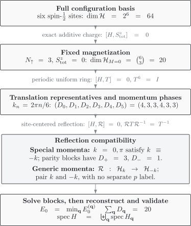
For a translation- and reflection-invariant six-site spin-$1/2$ ring, fixing $S^z_{\mathrm{tot}}=0$ reduces $64$ configurations to $20$. Translation gives momentum-block dimensions $(4,3,3,4,3,3)$. A site-centered reflection can refine the $k=0$ and $k=\pi$ blocks into parity dimensions $3+1$, but it exchanges generic $k$ and $-k$ sectors rather than supplying an additional parity label.

The order is practical, not a mathematical hierarchy. Additive charges reduce the candidate list before the more expensive orbit search. Spatial symmetries then reduce repeated configurations without ever constructing a full dense transformation.

Particle-Number Sectors

For $L$ modes,

$$\widehat N = \sum_{i=1}^{L} n_i.$$

If

$$[H,\widehat N]=0,$$

the Fock space decomposes as

$$\mathcal F = \bigoplus_N \mathcal H_N.$$

In an occupation basis, fixed-$N$ construction is direct: enumerate only configurations whose occupations sum to $N$.

For spinless fermions on $L$ orbitals,

$$\dim\mathcal H_N = \binom{L}{N}.$$

For bosons in $L$ modes with fixed total number and no additional local cutoff,

$$\dim\mathcal H_N = \binom{N+L-1}{N}.$$

For spinful fermions with separately conserved populations,

$$\dim \mathcal H_{N_{\uparrow},N_{\downarrow}} = \binom{L}{N_{\uparrow}} \, \binom{L}{N_{\downarrow}}.$$

These formulas count different model spaces. A local bosonic cutoff, forbidden double occupancy, gauge constraint, or orbital restriction changes the count and must be included before a dimension is used as a validation target.

Number conservation versus number parity

A pairing term such as

$$H_{\Delta} = \sum_{ij} \left( \Delta_{ij} c_i^{\dagger}c_j^{\dagger} + \Delta_{ij}^{*} c_jc_i \right)$$

changes particle number by two. Therefore

$$[H_{\Delta},\widehat N] \neq 0.$$

It can nevertheless preserve fermion-number parity,

$$\Pi_N = (-1)^{\widehat N}, \qquad [H_{\Delta},\Pi_N] = 0.$$

The correct blocks are then even and odd Fock-space sectors, not fixed-$N$ sectors. Confusing these two symmetries can remove physically required anomalous couplings.

Total Spin z-Component

For $L$ spin-$1/2$ sites,

$$S^z_{\mathrm{tot}} = \sum_{j=1}^{L} S_j^z.$$

If $N_{\uparrow}$ sites are up,

$$S^z_{\mathrm{tot}} = \hbar \left( N_{\uparrow} - \frac{L}{2} \right).$$

Thus a fixed-magnetization basis has dimension

$$D_{N_{\uparrow}} = \binom{L}{N_{\uparrow}}.$$

Exchange terms preserve this number because they move an up spin rather than create or destroy net magnetization:

$$S_i^{+}S_j^{-} : \quad N_{\uparrow} \longmapsto N_{\uparrow}.$$

The Heisenberg and XXZ chains conserve $S^z_{\mathrm{tot}}$. A transverse field generally does not:

$$\left[ \sum_j h_xS_j^x, S^z_{\mathrm{tot}} \right] \neq 0.$$

The fixed-$S^z_{\mathrm{tot}}$ basis is therefore model-dependent even when the local degrees of freedom are the same.

Fixed magnetization is not fixed total spin

For an $SU(2)$-invariant Hamiltonian,

$$[H,\mathbf S_{\mathrm{tot}}^2] = 0, \qquad [H,S^z_{\mathrm{tot}}] = 0.$$

A fixed-$M$ sector with

$$S^z_{\mathrm{tot}}|S,M\rangle = \hbar M|S,M\rangle$$

contains every total-spin multiplet satisfying $S\geq |M|$. Restricting to $M=0$ does not restrict to singlets. One may identify $S$ afterward from $\mathbf S_{\mathrm{tot}}^2$, construct a fully $SU(2)$-adapted basis, or use highest-weight counting. These routes have different implementation complexity.

Translation Momentum on a Periodic Cluster

Consider a periodic chain with $L$ sites and one-site translation $T$ satisfying

$$T^L=I.$$

Choose the convention

$$T|\psi_k\rangle = e^{-ik} |\psi_k\rangle.$$

The allowed dimensionless crystal momenta are

$$k_n = \frac{2\pi n}{L}, \qquad n=0,1,\ldots,L-1.$$

The momentum projector is

$$P_{k} = \frac{1}{L} \sum_{r=0}^{L-1} e^{ikr} T^r.$$

Translation is available only if $T$ maps the declared finite cluster, boundary conditions, local basis, and Hamiltonian coefficients onto themselves. A periodic drawing is not enough; the implemented bond list must be invariant.

Translation Orbits and Representatives

Start from a configuration $|a\rangle$ in an already filtered additive-charge sector. Its translation orbit is

$$\mathcal O_a = \left\{ |a\rangle, T|a\rangle, \ldots \right\}.$$

Let $R_a$ be the smallest positive integer satisfying

$$T^{R_a}|a\rangle = |a\rangle.$$

The orbit has $R_a$ distinct configurations. A deterministic convention, such as the smallest encoded integer, chooses one representative.

The normalized momentum state built from that orbit is

$$|a;k\rangle = \frac{1}{\sqrt{R_a}} \sum_{r=0}^{R_a-1} e^{ikr} T^r|a\rangle,$$

provided

$$e^{ikR_a} = 1.$$

If this compatibility condition fails, the projected state vanishes. This is the simplest stabilizer constraint: configurations with a shorter spatial period do not contribute to every momentum.

The momentum-block dimension can be checked independently from the character trace,

$$D_k = \operatorname{Tr}P_k = \frac{1}{L} \sum_{r=0}^{L-1} e^{ikr} \operatorname{Tr}_{\mathcal S} T^r,$$

where $\mathcal S$ is the prefiltered configuration space. The trace counts configurations fixed by each translation.

Worked Orbit Count for Six Spins

Take a six-site spin-$1/2$ ring at

$$N_{\uparrow}=3, \qquad S^z_{\mathrm{tot}}=0.$$

The fixed-magnetization dimension is

$$\binom{6}{3} = 20.$$

Eighteen configurations form three translation orbits of length six. The two Néel configurations

$$|\uparrow\downarrow\uparrow\downarrow \uparrow\downarrow\rangle, \qquad |\downarrow\uparrow\downarrow\uparrow \downarrow\uparrow\rangle$$

form one orbit of length two.

Each length-six orbit contributes one state to every $k_n$. The length-two orbit contributes only when

$$e^{i2k_n}=1,$$

which occurs for $n=0$ and $n=3$. Therefore

$$\left( D_0,D_1,D_2,D_3,D_4,D_5 \right) = \left( 4,3,3,4,3,3 \right).$$

The dimension ledger closes:

$$\sum_{n=0}^{5}D_n = 20.$$

Assuming every momentum block has dimension $20/6$ would have failed because orbit stabilizers make the blocks unequal.

Reflection and Parity

Let $\mathcal R$ be a reflection with

$$\mathcal R^2=I.$$

If

$$[H,\mathcal R]=0,$$

its eigenvalues are

$$p=\pm1.$$

In a basis where reflection is compatible with all previous labels, the projectors are

$$P_p = \frac{1}{2} \left( I+p\mathcal R \right).$$

For a one-dimensional periodic lattice, reflection reverses translation:

$$\mathcal R T \mathcal R^{-1} = T^{-1}.$$

Consequently,

$$\mathcal R : \quad \mathcal H_k \longrightarrow \mathcal H_{-k}.$$

Momentum and reflection parity can be imposed simultaneously only when

$$k \equiv -k \pmod{2\pi}.$$

Thus:

• $k=0$ always supports parity labels;
• $k=\pi$ supports parity labels when $L$ is even;
• generic $k$ and $-k$ are exchanged, so a single complex momentum block has no independent reflection-parity label.

At generic momentum one may retain separate complex $k$ and $-k$ blocks, combine them into a real two-component representation, or use a basis adapted to the appropriate dihedral-group irrep. One must not simply add a $p=\pm1$ label to each $k$ block.

For the six-site example and the site-centered reflection $j\mapsto -j$, each special momentum block splits as

$$\begin{aligned} k=0: &\qquad D_{+}=3, \quad D_{-}=1, \\ k=\pi: &\qquad D_{+}=3, \quad D_{-}=1. \end{aligned}$$

The split depends on the precisely defined reflection operation. Even rings have site-centered and bond-centered reflections related by a translation, and their labels can differ by a momentum-dependent phase.

Several meanings of parity

The word parity is overloaded in many-body work. Distinguish:

• spatial inversion or reflection;
• fermion-number parity $(-1)^{\widehat N}$;
• spin inversion, which flips every $S_j^z$;
• sublattice or chiral operations, which may anticommute rather than commute with $H$.

These operators have different algebras and different sectors. Name the operator, not only the eigenvalue.

Building a Reduced Hamiltonian Directly

Suppose $|a;\mathbf q\rangle$ are normalized symmetry-adapted states indexed by representatives. The block matrix is

$$\left( H_{\mathbf q} \right)_{ba} = \langle b;\mathbf q| H |a;\mathbf q\rangle.$$

A practical matrix-element kernel does the following:

1. take representative $a$;
2. apply one local Hamiltonian term to its underlying configuration;
3. reject outputs that violate an additive charge;
4. map each surviving output to its symmetry representative $b$;
5. record the group element used in that map;
6. multiply by its character or momentum phase;
7. include the orbit-normalization ratio;
8. accumulate the contribution in row $b$.

The phase convention and orbit normalization must be derived together. Reusing a phase from one translation convention with normalization from another can preserve plausible eigenvalues in special sectors while corrupting generic-momentum matrix elements.

For a matrix-free solver, the same representative map implements

$$x \longmapsto H_{\mathbf q}x$$

without storing the sparse block. The computational saving comes from never visiting equivalent configurations as independent basis vectors.

Complex arithmetic is sometimes physical bookkeeping

For generic momentum,

$$e^{ikr} \notin \mathbb R.$$

The reduced Hamiltonian may therefore be complex Hermitian even when the original configuration-basis Hamiltonian is real. Discarding imaginary parts does not make the calculation more exact; it changes the representation. Real formulations exist by pairing $k$ and $-k$, but they require the corresponding two-component basis.

Observables Can Change Sectors

A Hamiltonian-preserving label need not be preserved by every observable.

If an additive charge satisfies

$$[Q,O] = \Delta q\,O,$$

then

$$P_{q'} O P_q = 0 \quad \text{unless} \quad q'=q+\Delta q.$$

An annihilation operator connects $N$ to $N-1$. A spin-raising operator connects magnetization sectors differing by $\hbar$. A momentum-resolved operator satisfying

$$T O_p T^{-1} = e^{-ip}O_p$$

maps

$$\mathcal H_k \longrightarrow \mathcal H_{k+p}.$$

An operator odd under reflection connects opposite parity sectors at compatible momentum.

This matters for spectral functions. A ground state may be computed in one sector, while every intermediate state contributing to a response lies in another. Restricting both sides of the matrix element to the ground-state block can force the desired signal to zero by construction.

Ground States Require a Cross-Sector Search

Let

$$E_0^{(\mathbf q)} = \min \operatorname{spec} H_{\mathbf q}.$$

The unconstrained finite-system ground-state energy is

$$E_0 = \min_{\mathbf q} E_0^{(\mathbf q)}.$$

Solving one convenient block establishes only the ground state within that block. It does not establish the global ground state unless a theorem or an explicit cross-sector comparison identifies the winning label.

This distinction is especially important when:

• a coupling drives a level crossing between different symmetry sectors;
• the first excitation lies at momentum different from the ground state;
• boundary conditions reorder low-energy levels;
• a magnetic field changes the favored magnetization;
• a pairing problem requires comparing even and odd number parity;
• finite clusters in a sequence admit different momentum grids.

Crossings between distinct exact sectors can be sharp because the states cannot hybridize. Levels with identical complete symmetry labels generically repel unless another conservation law or integrable structure intervenes.

Finite Symmetry and Spontaneous Symmetry Breaking

A finite Hamiltonian with an exact symmetry can be diagonalized in symmetry sectors even when its thermodynamic phase breaks that symmetry.

Finite eigenstates normally carry definite symmetry labels. A symmetry-broken configuration is then represented by a superposition of low-lying states from different sectors. The thermodynamic pattern is inferred from:

• near-degenerate parity doublets;
• towers of states in several spin sectors;
• low-energy levels at ordering momenta;
• order-parameter correlations and structure factors;
• systematic scaling with size and geometry.

Selecting one broken-symmetry product state and calling it the exact finite ground state discards the finite-system symmetry structure that carries the scaling evidence.

Thermal Traces Across Sectors

For a complete orthogonal decomposition,

$$Z(\beta) = \operatorname{Tr} e^{-\beta H} = \sum_{\mathbf q} \operatorname{Tr}_{\mathcal H_{\mathbf q}} e^{-\beta H_{\mathbf q}}.$$

If an observable preserves every sector,

$$\langle O\rangle_{\beta} = \frac{1}{Z} \sum_{\mathbf q} \operatorname{Tr}_{\mathcal H_{\mathbf q}} \left( e^{-\beta H_{\mathbf q}} O_{\mathbf q} \right).$$

One-sector thermodynamics is a constrained ensemble unless the physical preparation fixes that sector.

For non-Abelian reductions, record whether the numerical block retains every irrep row or only a multiplicity space. If only one repeated block is solved, the irrep dimension must be restored in full traces.

Spectral Statistics Must Be Desymmetrized

Level-spacing statistics compare neighboring eigenvalues that are allowed to repel. Combining independent exact sectors superposes unrelated spectra. Cross-sector crossings then produce many small spacings and can mimic Poisson-like behavior even when each irreducible block has random-matrix correlations.

A defensible level-statistics calculation therefore fixes:

• particle number or magnetization;
• translation momentum;
• every compatible point-group or reflection label;
• number parity or spin inversion where applicable;
• any remaining exact conservation law;
• an energy window and unfolding or spacing-ratio convention.

The Many-Body Quantum Chaos Preview owns the physical interpretation. Here the key numerical rule is simple: compare levels only after all exact unitary symmetries have been resolved as far as the analysis requires.

Dimension and Closure Checks

Every sector implementation should pass a dimension ledger:

$$\sum_{\mathbf q} D_{\mathbf q} = D_{\mathrm{parent}}.$$

For nested reductions, check the equality at each stage:

$$D_{\mathrm{full}} \longrightarrow \sum_N D_N \longrightarrow \sum_{N,k}D_{N,k} \longrightarrow \sum_{N,k,p}D_{N,k,p}.$$

Only compatible parity labels belong in the final sum.

Projector closure can be tested by random vectors:

$$\epsilon_{\mathrm{leak}}(x) = \frac{ \left\| (I-P_{\mathbf q}) H P_{\mathbf q}x \right\| }{ \left\| H P_{\mathbf q}x \right\| + \epsilon }.$$

A symmetry-action test is

$$\epsilon_g(x) = \frac{ \left\| HU_gx-U_gHx \right\| }{ \left\| HU_gx \right\| + \left\| U_gHx \right\| + \epsilon }.$$

Both should scale with numerical roundoff for an exact implemented symmetry.

Spectral and Trace Reconstruction

On a small system where the unreduced calculation is feasible, the union of block spectra must equal the full spectrum with multiplicity:

$$\operatorname{spec}H = \biguplus_{\mathbf q} \operatorname{spec}H_{\mathbf q}.$$

Low-order trace moments provide basis-independent tests:

$$\begin{aligned} \operatorname{Tr}H &= \sum_{\mathbf q} \operatorname{Tr}H_{\mathbf q}, \\ \operatorname{Tr}H^2 &= \sum_{\mathbf q} \operatorname{Tr}H_{\mathbf q}^2. \end{aligned}$$

The first catches missing diagonal contributions and missing blocks. The second is sensitive to off-diagonal amplitudes, phase factors, and normalization.

Additional checks include:

• Hermiticity of every block;
• representative uniqueness;
• group multiplication on encoded configurations;
• orbit length dividing the group order;
• vanishing of incompatible projected states;
• expected $k\leftrightarrow -k$ spectral pairing when a reflection or suitable antiunitary symmetry is present;
• agreement of symmetry-resolved observables reconstructed from the full eigenvectors.

A Reproducible Sector Record

For each reported block, save:

• finite geometry and boundary conditions;
• basis ordering and local encoding;
• parent-space constraints;
• explicit symmetry maps on sites or modes;
• quantum-number conventions and allowed values;
• representative rule;
• orbit or stabilizer data;
• block dimension;
• whether arithmetic is real or complex;
• closure and Hermiticity residuals;
• independent dimension and trace checks;
• the set of sectors searched for the reported physical conclusion.

A label such as “$k=0$ even sector” is not reproducible until the translation direction, reflection axis, phase convention, and parent charge sector are specified.

Common Mistakes

Assuming the infinite model’s symmetry survives the cluster

An open boundary, irregular cluster, twist, impurity, or gauge convention can change the finite symmetry group.

Dividing dimensions by the group order

Short orbits and fixed configurations make symmetry blocks unequal. Use orbit stabilizers or character traces.

Combining noncommuting labels

Reflection and generic momentum are the standard example. Both commute with $H$, but reflection exchanges $k$ and $-k$.

Confusing $S^z_{\mathrm{tot}}$ with total spin

A magnetization block contains several $S$ multiplets unless a fully $SU(2)$-adapted basis is used.

Confusing fixed number with number parity

Pairing terms preserve $(-1)^{\widehat N}$ while mixing different $N$ values.

Dropping orbit normalization factors

Representatives with different stabilizers have different orbit lengths. Treating them identically corrupts matrix elements.

Forcing a generic momentum block to be real

Complex phases are part of the one-dimensional translation representation. A real basis requires pairing $k$ with $-k$ consistently.

Searching only one sector

The lowest state of a selected block need not be the global ground state or first excitation.

Evaluating a sector-changing observable inside one block

Creation, annihilation, spin-flip, and finite-momentum operators require target sectors with shifted labels.

Mixing sectors in level statistics

Independent spectra do not repel. Their superposition can imitate a different dynamical regime.

Trusting a library label without checking conventions

Software packages differ in site ordering, translation direction, parity map, eigenvalue convention, and whether a label denotes an eigenvalue or an integer index.

Exercises

1. Translation blocks for six spins

In the $N_{\uparrow}=3$ sector of a six-site ring, suppose there are three translation orbits of length six and one orbit of length two.

1. Find the dimension of each momentum block.
2. Verify that the dimensions sum to $\binom{6}{3}$.
3. Explain why the length-two orbit contributes only at $k=0$ and $k=\pi$.

Solution

Each length-six orbit contributes one normalized projected state to every allowed momentum

$$k_n = \frac{2\pi n}{6}.$$

The length-two orbit is compatible only if

$$e^{i2k_n} = 1.$$

Thus

$$n=0 \quad \text{or} \quad n=3.$$

The three generic orbits contribute three states to every sector, and the short orbit adds one at those two momenta:

$$\left( D_0,D_1,D_2,D_3,D_4,D_5 \right) = \left( 4,3,3,4,3,3 \right).$$

Finally,

$$4+3+3+4+3+3 = 20 = \binom{6}{3}.$$

2. Why generic momentum has no reflection parity

Let

$$\mathcal R T \mathcal R^{-1} = T^{-1}.$$

Assume a nonzero state is simultaneously an eigenstate of $T$ and $\mathcal R$:

$$T|\psi\rangle = e^{-ik}|\psi\rangle, \qquad \mathcal R|\psi\rangle = p|\psi\rangle.$$

Determine the allowed momenta.

Solution

Act with $T$ on the reflected state:

$$\begin{aligned} T\mathcal R|\psi\rangle &= \mathcal R T^{-1}|\psi\rangle \\ &= e^{ik} \mathcal R|\psi\rangle. \end{aligned}$$

But $\mathcal R|\psi\rangle=p|\psi\rangle$, so the same nonzero vector would have translation eigenvalues $e^{-ik}$ and $e^{ik}$. Therefore

$$e^{-ik} = e^{ik},$$

or

$$e^{i2k}=1.$$

Hence

$$k=0 \quad \text{or} \quad k=\pi \pmod{2\pi}.$$

The $k=\pi$ value belongs to the finite momentum grid only when $L$ is even.

3. Pairing preserves parity but not number

Consider

$$H_{\Delta} = \Delta c_1^{\dagger}c_2^{\dagger} + \Delta^{*} c_2c_1.$$

Show that $H_{\Delta}$ does not conserve $\widehat N$ but does conserve $\Pi_N=(-1)^{\widehat N}$.

Solution

The number-operator commutators are

$$\begin{aligned} \left[ \widehat N, c_1^{\dagger}c_2^{\dagger} \right] &= 2c_1^{\dagger}c_2^{\dagger}, \\ \left[ \widehat N, c_2c_1 \right] &= -2c_2c_1. \end{aligned}$$

Therefore

$$\left[ \widehat N, H_{\Delta} \right] \neq 0$$

for nonzero $\Delta$.

Number parity acts on a single fermion operator as

$$\Pi_N c_i^{\dagger}\Pi_N^{-1} = -c_i^{\dagger}, \qquad \Pi_N c_i\Pi_N^{-1} = -c_i.$$

Every pairing monomial contains two such operators, so the two minus signs cancel:

$$\Pi_N H_{\Delta}\Pi_N^{-1} = H_{\Delta}.$$

Thus the Hamiltonian mixes $N$ with $N\pm2$ but never mixes even and odd $N$.

4. Momentum carried by an observable

Let local operators translate according to

$$T O_j T^{-1} = O_{j+1},$$

and define

$$O_q = \frac{1}{\sqrt L} \sum_{j=0}^{L-1} e^{iqj} O_j.$$

Show that $O_q$ maps momentum $k$ to momentum $k+q$.

Solution

Translate the Fourier component:

$$\begin{aligned} T O_q T^{-1} &= \frac{1}{\sqrt L} \sum_j e^{iqj} O_{j+1} \\ &= e^{-iq} \frac{1}{\sqrt L} \sum_{\ell} e^{iq\ell} O_{\ell} \\ &= e^{-iq}O_q. \end{aligned}$$

For

$$T|\psi_k\rangle = e^{-ik}|\psi_k\rangle,$$

one obtains

$$\begin{aligned} T O_q|\psi_k\rangle &= \left( T O_qT^{-1} \right) T|\psi_k\rangle \\ &= e^{-i(k+q)} O_q|\psi_k\rangle. \end{aligned}$$

Therefore

$$O_q : \quad \mathcal H_k \longrightarrow \mathcal H_{k+q}.$$

5. Magnetization does not determine total spin

Four spin-$1/2$ degrees of freedom decompose into two spin-zero multiplets, three spin-one multiplets, and one spin-two multiplet. Determine the dimension and total-spin content of the $M=0$ sector.

Solution

Every integer-spin multiplet contains exactly one state with $M=0$. Therefore the $M=0$ sector contains:

• two states from the two singlet multiplets;
• three states from the three triplet multiplets;
• one state from the quintet multiplet.

Its dimension is

$$D_{M=0} = 2+3+1 = 6.$$

This agrees with direct fixed-magnetization counting:

$$D_{M=0} = \binom{4}{2} = 6.$$

The equality confirms the count, while the decomposition shows why $M=0$ cannot be used as a synonym for $S=0$.

References

• H. Q. Lin, “Exact Diagonalization of Quantum-Spin Models,” Physical Review B 42, 6561–6567 (1990), doi:10.1103/PhysRevB.42.6561.
• A. W. Sandvik, “Computational Studies of Quantum Spin Systems,” in AIP Conference Proceedings 1297, 135–338 (2010), doi:10.1063/1.3518900.
• A. Wietek and A. M. Läuchli, “Sublattice Coding Algorithm and Distributed Memory Parallelization for Large-Scale Exact Diagonalizations of Quantum Many-Body Systems,” Physical Review E 98, 033309 (2018), doi:10.1103/PhysRevE.98.033309.
• P. Weinberg and M. Bukov, “QuSpin: A Python Package for Dynamics and Exact Diagonalisation of Quantum Many Body Systems, Part I: Spin Chains,” SciPost Physics 2, 003 (2017), doi:10.21468/SciPostPhys.2.1.003.
• P. Weinberg and M. Bukov, “QuSpin: A Python Package for Dynamics and Exact Diagonalisation of Quantum Many Body Systems, Part II: Bosons, Fermions and Higher Spins,” SciPost Physics 7, 020 (2019), doi:10.21468/SciPostPhys.7.2.020.
• T. Westerhout, “lattice-symmetries: A Package for Working with Quantum Many-Body Bases,” Journal of Open Source Software 6, 3537 (2021), doi:10.21105/joss.03537.
• E. Dagotto, “Correlated Electrons in High-Temperature Superconductors,” Reviews of Modern Physics 66, 763–840 (1994), doi:10.1103/RevModPhys.66.763.
• H. Fehske, R. Schneider, and A. Weiße, eds., Computational Many-Particle Physics, Springer, 2008, doi:10.1007/978-3-540-74686-7.
• M. Tinkham, Group Theory and Quantum Mechanics, Dover, 2003.

Further Study

• Computational Many-Body Overview
• Exact Diagonalization Preview
• Lanczos Method Preview
• Scaling of Hilbert Space
• Many-Body Hilbert Spaces Overview
• Number Operators and Conserved Quantities
• Boundary Conditions on Lattices
• Translation-Invariant Hamiltonians
• Parity
• Heisenberg Model
• Sparse Eigensolvers
• Many-Body Quantum Chaos Preview
• Validation Tests