Many-Body Hilbert Spaces Overview

A many-body Hilbert space is the state space obtained after declaring which degrees of freedom exist, whether particles are distinguishable, which exchange statistics apply, whether particle number is fixed, and which constraints or cutoffs are imposed. It is part of the physical model, not merely a container chosen after the Hamiltonian is written.

The same verbal system can lead to different spaces. “Two particles in four orbitals” could mean two labeled particles in $\mathbb C^4\otimes\mathbb C^4$, two bosons in $\operatorname{Sym}^2\mathbb C^4$, or two fermions in $\bigwedge^2\mathbb C^4$. Those spaces have dimensions $16$, $10$, and $6$, respectively. They encode different physical assumptions before any interaction is specified.

The main structures used in many-body quantum mechanics are

$$\begin{aligned} \text{labeled particles:} &\quad \mathcal h^{\otimes N}, \\ \text{identical bosons:} &\quad \operatorname{Sym}^N\mathcal h, \\ \text{identical fermions:} &\quad \bigwedge^N\mathcal h, \\ \text{variable particle number:} &\quad \mathcal F_\pm(\mathcal h), \\ \text{local lattice degrees of freedom:} &\quad \bigotimes_{i=1}^{L}\mathcal h_i. \end{aligned}$$

Symmetries and constraints then select direct-sum blocks or physical subspaces inside these larger spaces.

Choosing a many-body Hilbert space means deciding what can coexist, what counts as the same physical configuration, and which sectors the dynamics may connect.

The foundational definitions of tensor products, exchange symmetry, Fock space, and second quantization live in Composite Systems and Entanglement. This page owns their use as a many-body modeling decision: selecting sectors, matching ensembles, identifying equivalent representations, keeping lattice and particle constructions distinct, and documenting truncations. Scaling of Hilbert Space owns detailed dimension counts and asymptotics.

Start with Four Questions

Before writing a basis or Hamiltonian, answer four questions.

1. What are the elementary degrees of freedom? Examples include particle position and spin, lattice-site spins, orbitals, bands, species, phonon modes, or gauge-constrained links.
2. How are they combined? Simultaneous distinguishable factors use tensor products. Alternative sectors use direct sums. Identical particles require symmetric or antisymmetric sectors.
3. What is fixed or conserved? Particle number, total spin projection, momentum, charge, parity, and other quantum numbers can restrict the working space.
4. What has been truncated? Finite volume, mode cutoff, local occupation cutoff, energy window, and symmetry selection all change the represented Hilbert space.

A complete model statement identifies all four. Naming only a basis is insufficient because the same Hilbert space admits many bases, and the same tuple notation can be used for inequivalent spaces.

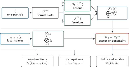
The main many-body constructions. Identical-particle fixed-$N$ sectors are selected from $\mathcal h^{\otimes N}$ by exchange symmetry and collected by a direct sum in Fock space. Local spins or truncated on-site variables instead begin with a tensor product over distinguishable sites. Conserved quantities and physical constraints select blocks $\mathcal H_q$ in either construction. Coordinate wavefunctions, occupation tuples, momentum states, and field operators are representations or operator languages on these spaces, not four new physical Hilbert spaces.

The One-Particle Hilbert Space

For particle-based problems, the starting object is a one-particle Hilbert space $\mathcal h$. A continuum particle with position, spin, and perhaps an orbital or species label may have

$$\mathcal h = L^2(\Omega,d^dr) \otimes \mathbb C^{g_{\mathrm{spin}}} \otimes \mathbb C^{g_{\mathrm{internal}}}.$$

The factors describe simultaneous one-particle degrees of freedom. A basis vector might be labeled by

$$\lvert\alpha\rangle = \lvert\mathbf r,\sigma,a\rangle,$$

or by momentum, band, and spin labels,

$$\lvert\alpha\rangle = \lvert\mathbf k,n,\sigma\rangle.$$

These are different bases or representations of the same declared one-particle model when connected by a unitary transformation. A finite calculation usually replaces $\mathcal h$ by a retained subspace

$$\mathcal h_M = \operatorname{span} \left\{ \lvert\varphi_1\rangle, \ldots, \lvert\varphi_M\rangle \right\}.$$

The integer $M$ then counts one-particle modes, including all internal labels. A spatial orbital with spin up and the same spatial orbital with spin down are two distinct spin-orbitals.

Species require another declaration

Different species can be represented by separate one-particle spaces. For two distinguishable species $A$ and $B$ with fixed particle numbers,

$$\mathcal H = \mathcal H_{N_A}^{(A)} \otimes \mathcal H_{N_B}^{(B)}.$$

Exchange symmetry is imposed within each identical species, not between physically distinguishable species. If conversion processes change species labels, a larger direct-sum or Fock-space description may be required.

Labeled Fixed-Particle Spaces

For $N$ distinguishable particles sharing the same one-particle space, the formal state space is

$$\mathcal H_N^{\mathrm{lab}} = \mathcal h^{\otimes N}.$$

A product basis has vectors

$$\lvert\alpha_1\rangle_1 \otimes \cdots \otimes \lvert\alpha_N\rangle_N.$$

The subscripts identify independently addressable particles or formal slots. For genuinely distinguishable particles, local operations can act on one factor without being required to act on the others.

If $\dim\mathcal h=M<\infty$, then

$$\dim\mathcal H_N^{\mathrm{lab}} = M^N.$$

This full tensor product is also a useful temporary construction for identical particles because permutation operators act naturally on its slots. The physical identical-particle space is a restricted subspace, not the full slot-labeled tensor product.

Identical-Particle Fixed-N Sectors

Let $U(\pi)$ permute the $N$ tensor slots according to $\pi\in S_N$. The bosonic and fermionic projectors are

$$P_+ = \frac{1}{N!} \sum_{\pi\in S_N} U(\pi),$$

and

$$P_- = \frac{1}{N!} \sum_{\pi\in S_N} \operatorname{sgn}(\pi) U(\pi).$$

The physical fixed-number spaces are

$$\mathcal H_N^{(+)} = P_+\mathcal h^{\otimes N} = \operatorname{Sym}^N\mathcal h$$

for bosons, and

$$\mathcal H_N^{(-)} = P_-\mathcal h^{\otimes N} = \bigwedge^N\mathcal h$$

for fermions.

Particle-slot labels remain useful as coordinate arguments, but they are not persistent particle identities. An observable for identical particles must respect the exchange structure. The Symmetrization Postulate owns the foundational statement and its assumptions.

For a finite $M$-mode one-particle space,

$$\dim\operatorname{Sym}^N\mathcal h_M = \binom{N+M-1}{N},$$

whereas

$$\dim\bigwedge^N\mathcal h_M = \binom{M}{N}.$$

The fermionic sector is zero for $N>M$. This is Pauli exclusion expressed as a statement about the exterior power.

Fixed N versus Fock Space

A fixed-particle calculation needs only one sector $\mathcal H_N^{(\pm)}$. Fock space collects all allowed particle-number sectors:

$$\mathcal F_\pm(\mathcal h) = \bigoplus_{N=0}^{\infty} \mathcal H_N^{(\pm)}.$$

A Fock-space vector is a sector sequence

$$\lvert\Psi\rangle = \bigoplus_{N=0}^{\infty} \lvert\psi_N\rangle,$$

with

$$\sum_{N=0}^{\infty} \lVert\psi_N\rVert^2 < \infty.$$

This direct sum has a different structural meaning from a tensor product. Values of $N$ label orthogonal alternatives, not simultaneously present subsystems. The page Direct Sums versus Tensor Products owns that distinction.

When Fock space is useful

Fock space is natural when:

• creation and annihilation operators are used;
• a reservoir exchanges particles with the system;
• pairing or source terms connect number sectors;
• a grand-canonical ensemble is convenient;
• particles are excitations of modes rather than permanently labeled objects;
• one wants one operator language that acts consistently across all fixed-$N$ sectors.

Fock space does not imply that the physical state has indefinite particle number. A number eigenstate belongs to Fock space but has support in only one sector. A number-conserving Hamiltonian is block diagonal on Fock space and can be restricted to a fixed-$N$ block.

The canonical construction of bosonic and fermionic Fock spaces lives in Fock Space and Occupation Number. The present volume applies that construction to gases, lattices, response functions, and many-body approximations.

Local Tensor-Product Systems

Not every many-body problem begins with identical particles. A spin model assigns a local Hilbert space $\mathcal h_i$ to each distinguishable site $i$. For $L$ sites,

$$\mathcal H_{\mathrm{lat}} = \bigotimes_{i=1}^{L} \mathcal h_i.$$

For a spin-$s$ degree of freedom,

$$\dim\mathcal h_i = 2s+1.$$

A spin-$1/2$ chain therefore has

$$\mathcal H_L = (\mathbb C^2)^{\otimes L}, \qquad \dim\mathcal H_L = 2^L.$$

The tensor factors are sites, not particle labels. A local spin flip acts on one site factor. Exchange statistics is not imposed by symmetrizing the site tensor product.

This distinction matters for entanglement. A spatial cut of a spin chain naturally partitions site factors. An identical-particle problem requires a declared mode, region, or observable-algebra partition before an entanglement claim has operational meaning.

Lattice Particles and Equivalent Finite Constructions

Particle and site viewpoints can describe the same finite lattice model in different languages.

For a spinful fermion orbital at one site, the local states are

$$\lvert0\rangle, \quad \lvert\uparrow\rangle, \quad \lvert\downarrow\rangle, \quad \lvert\uparrow\downarrow\rangle.$$

The local space has dimension four, so $L$ sites give

$$\mathcal H_{\mathrm{site}} = (\mathbb C^4)^{\otimes L}, \qquad \dim\mathcal H_{\mathrm{site}} = 4^L.$$

The same finite system can be described as the fermionic Fock space of $2L$ ordered spin-orbitals:

$$\mathcal F_-(\mathbb C^{2L}), \qquad \dim\mathcal F_-(\mathbb C^{2L}) = 2^{2L} = 4^L.$$

The vector-space dimensions match, but fermionic operator ordering and graded signs must be handled consistently. A naive site tensor product does not erase the anticommutation algebra. Jordan–Wigner strings in one dimension are one way those signs reappear when fermions are represented by ordinary spin operators.

For lattice bosons, each site has infinitely many occupation states unless a local cutoff $n_i\le n_{\max}$ is imposed. With that numerical cutoff,

$$\mathcal H_{\mathrm{trunc}} = \bigotimes_{i=1}^{L} \mathbb C^{n_{\max}+1},$$

and

$$\dim\mathcal H_{\mathrm{trunc}} = (n_{\max}+1)^L.$$

That is a computational approximation unless the microscopic model itself has a finite local occupancy.

Symmetry Sectors and Conserved Blocks

Suppose a self-adjoint operator $Q$ has spectral subspaces $\mathcal H_q$. In a discrete finite-dimensional setting,

$$\mathcal H = \bigoplus_q \mathcal H_q.$$

If

$$[H,Q] = 0,$$

then the Hamiltonian preserves each sector:

$$H\mathcal H_q \subseteq \mathcal H_q.$$

Writing $P_q$ for the projector onto $\mathcal H_q$,

$$H = \bigoplus_q H_q, \qquad H_q = P_qHP_q.$$

Typical labels include particle number, magnetization, crystal momentum, parity, total angular momentum, and irreducible representation labels.

Working in one sector has three benefits:

• it enforces the desired physical constraint exactly;
• it reduces the matrix dimension;
• it prevents numerical mixing between quantum numbers that the exact dynamics conserves.

Not every useful basis simultaneously diagonalizes every symmetry. Noncommuting conserved quantities require compatible labels, such as total $S^2$ together with one spin component $S_z$.

Constraints Are More Than Convenient Blocks

Some physical state spaces are kernels or projected subspaces defined by constraints:

$$\mathcal H_{\mathrm{phys}} = \left\{ \lvert\Psi\rangle\in\mathcal H_{\mathrm{kin}}: G_a\lvert\Psi\rangle=0 \text{ for every }a \right\}.$$

Examples include hard constraints on local occupancy, fixed total charge, gauge constraints, and effective models that exclude high-energy configurations.

Three ideas should be separated:

1. a conserved sector is preserved by a specified Hamiltonian;
2. a physical constraint declares some kinematic vectors unphysical in the model;
3. a superselection restriction limits accessible coherence or observables between sectors.

The equation $[H,Q]=0$ proves conservation under that Hamiltonian. It does not by itself prove a universal superselection rule. Particle-Number Superselection Preview owns the operational distinction.

Representations Do Not Change the Physical Space

A Hilbert space can be described in coordinate, momentum, occupation, energy-eigenstate, tensor-network, or other bases. These choices change the coordinates of states and operators, not the underlying physical state space when the transformation is unitary and complete.

For a fixed-$N$ state,

$$\Psi(x_1,\ldots,x_N) = \langle x_1,\ldots,x_N\vert\Psi\rangle$$

is its coordinate representation. In a mode basis,

$$\lvert\Psi\rangle = \sum_{\boldsymbol n} C_{\boldsymbol n} \lvert\boldsymbol n\rangle.$$

In a field-operator language, the same state can be constructed by applying smeared creation fields to the vacuum.

The representations emphasize different structures:

Language	Natural labels	Best suited to
first-quantized wavefunction	particle slots and one-particle coordinates	fixed small $N$, coordinate-space boundary conditions
occupation-number basis	mode populations	exchange symmetry, sparse operators, exact diagonalization
momentum-space basis	mode momenta and internal labels	translation invariance, Fermi surfaces, scattering
real-space fields	position and internal labels	local densities, continuum interactions, correlations
local tensor basis	site configurations	spin systems, lattice locality, tensor networks

First-Quantized Many-Body Wavefunctions owns the coordinate-space construction. Occupation-Number Representation owns practical mode-basis construction and sparse calculations. Field Operators in Many-Body Models owns the continuum operator language.

First Quantization and Second Quantization

The names can suggest two different quantum theories. In ordinary nonrelativistic many-body mechanics, they are usually equivalent descriptions sector by sector.

For a normalized bosonic or fermionic wavefunction $\Psi(x_1,\ldots,x_N)$, one may write

$$\lvert\Psi_N\rangle = \frac{1}{\sqrt{N!}} \int dx_1\cdots dx_N\, \Psi(x_1,\ldots,x_N) \psi^\dagger(x_1) \cdots \psi^\dagger(x_N) \lvert0\rangle.$$

Exchange symmetry is carried explicitly by $\Psi$ in first quantization and by the field algebra in the operator construction. The physical information agrees when conventions and normalizations match.

Second quantization becomes especially efficient when particle number varies, but its operator language remains useful in one fixed-number sector. The second-quantization chapter owns the foundational operator construction.

Worked Example: Two Fermions in Three Modes

Let

$$\mathcal h_3 = \operatorname{span} \left\{ \lvert1\rangle, \lvert2\rangle, \lvert3\rangle \right\}.$$

The two-fermion physical space is

$$\mathcal H_2^{(-)} = \bigwedge^2\mathcal h_3,$$

with dimension

$$\binom{3}{2} = 3.$$

An occupation basis is

$$\lvert110\rangle, \qquad \lvert101\rangle, \qquad \lvert011\rangle.$$

The corresponding first-quantized basis wavefunctions are the normalized antisymmetric pairs

$$\lvert i\wedge j\rangle = \frac{1}{\sqrt2} \left( \lvert i\rangle_1\lvert j\rangle_2 - \lvert j\rangle_1\lvert i\rangle_2 \right),$$

for $(i,j)=(1,2),(1,3),(2,3)$. Occupation notation has not added or removed states; it has encoded antisymmetry once in the basis convention.

The full fermionic Fock space over three modes has dimension $2^3=8$. It includes the vacuum, three one-particle states, these three two-particle states, and one three-particle state. A fixed-$N=2$ Hamiltonian need not carry the other five states.

Worked Example: Two Spin-1/2 Fermions in Two Orbitals

Let the spatial orbitals be $a$ and $b$. Including spin, the one-particle modes are

$$a\uparrow, \quad a\downarrow, \quad b\uparrow, \quad b\downarrow.$$

Thus

$$\dim\mathcal h = 4.$$

The two-fermion sector has dimension

$$\dim\bigwedge^2\mathcal h = \binom42 = 6.$$

Two basis states have double occupancy of one spatial orbital,

$$\lvert a\uparrow,a\downarrow\rangle, \qquad \lvert b\uparrow,b\downarrow\rangle,$$

and four have one fermion in each orbital. Recombining the latter into total-spin singlet and triplet combinations is another basis change inside the same six-dimensional space.

This example shows why “two orbitals” does not mean $M=2$ when spin is an active one-particle label.

Operators Must Match the Space

An operator is not specified by a symbolic formula alone. Its domain, codomain, statistics, and sector action matter.

For a one-particle operator $A$ with matrix elements $A_{ij}$, its number-conserving lift to Fock space has the pattern

$$d\Gamma(A) = \sum_{ij} A_{ij} a_i^\dagger a_j.$$

It preserves particle number because each term annihilates and creates one particle. A pairing term such as

$$\Delta_{ij} a_i^\dagger a_j^\dagger + \Delta_{ij}^* a_j a_i$$

connects sectors whose particle numbers differ by two and therefore cannot act within one fixed-$N$ space by itself.

On a site tensor product, a local operator is embedded as

$$O_i = I_1\otimes\cdots\otimes I_{i-1} \otimes O \otimes I_{i+1}\otimes\cdots\otimes I_L.$$

The One-Body Operators and Two-Body Operators application guides develop matrix elements, reduced density matrices, interaction conventions, and computational checks. This overview uses those structures only to show how operator form reveals the required Hilbert space.

Pure States, Mixed States, and Ensembles

Choosing a Hilbert space does not choose a state. A pure state is a ray represented by $\lvert\Psi\rangle\in\mathcal H$. A mixed state is represented by a positive trace-one operator $\rho$ acting on the same physical space or sector.

For fixed particle number,

$$\rho_N = \frac{e^{-\beta H_N}}{Z_N}, \qquad Z_N = \operatorname{Tr}_{\mathcal H_N} e^{-\beta H_N}.$$

For a grand-canonical description on Fock space,

$$\rho_{\mathrm{GC}} = \frac{ e^{-\beta(H-\mu N)} }{ \Xi },$$

with

$$\Xi = \operatorname{Tr}_{\mathcal F} e^{-\beta(H-\mu N)}.$$

If $[H,N]=0$, this density operator is block diagonal in particle number. Grand-canonical number fluctuations do not require coherent pure-state superpositions of different $N$; they can arise from a classical mixture of number sectors.

The Canonical Ensemble and Grand Canonical Ensemble pages own the thermodynamic constructions and their equivalence conditions.

Truncation Is Part of the Model Statement

Continuum and bosonic Hilbert spaces are usually infinite-dimensional. Numerical work replaces them by a finite subspace. Common cutoffs include:

• a finite spatial volume;
• a finite one-particle basis of $M$ modes;
• a momentum or energy cutoff;
• a maximum local boson occupation $n_{\max}$;
• a maximum total excitation or particle number;
• a selected symmetry sector;
• an active-space restriction around a reference configuration.

Let $P_\Lambda$ project onto the retained subspace. The simplest projected Hamiltonian is

$$H_\Lambda = P_\Lambda H P_\Lambda.$$

This expression does not guarantee controlled accuracy. Eliminated states can renormalize couplings, generate new operators, or produce energy-dependent effective interactions. A trustworthy calculation states:

1. what $\Lambda$ means;
2. which observables are expected to be insensitive to it;
3. how convergence is tested as the retained space grows;
4. whether couplings have been matched or renormalized at that cutoff;
5. which symmetries the truncation preserves or breaks.

A local occupation cutoff that changes a result when increased is not a harmless implementation detail. It is an unresolved approximation error.

Basis Changes and Truncations Do Not Commute Automatically

Suppose $U$ is a unitary basis change on the full one-particle space. If $P_M$ selects $M$ retained modes, then in general

$$P_MU \ne UP_M.$$

Truncating localized orbitals and truncating energy eigenmodes can therefore produce different finite models even when the complete bases span the same infinite-dimensional space.

This is why one should distinguish:

• a unitary representation change in a complete space;
• a projection to a finite active subspace;
• an effective model obtained after integrating out excluded states.

Only the first is automatically an exact reformulation.

Finite Volume and the Thermodynamic Limit

At finite volume or finite lattice size, one can usually specify an ordinary Hilbert space $\mathcal H_L$ and Hamiltonian $H_L$. The thermodynamic limit is a sequence

$$(\mathcal H_L,H_L) \quad\text{with}\quad L,N,V\to\infty$$

under a declared scaling, such as fixed density.

It is often misleading to imagine that every infinite system is simply one enormous tensor product with all finite-volume vectors embedded uniquely. In the infinite limit:

• physically relevant states may be defined through expectation values of local observables;
• distinct phases can lead to inequivalent Hilbert-space representations;
• symmetry-broken states can emerge only after the order of limits and source removal is specified;
• thermal states need not be represented by trace-class density matrices on a naive infinite-volume space.

Finite-volume calculations remain the controlled starting point. The Thermodynamic Limit page owns limiting procedures, boundary effects, and noncommuting limits. Operator-algebraic infinite-system constructions are an advanced extension, not assumed silently in finite-model formulas.

Locality Depends on the Factorization

An operator is local only relative to a declared decomposition.

For a lattice tensor product, “local” commonly means support on a bounded set of sites. In a continuum field theory, it means an operator density smeared over a spatial region. In a momentum basis, the same real-space local interaction may connect many momenta. In an energy eigenbasis, even a simple local observable can be dense.

Similarly, entanglement depends on a subsystem or algebra decomposition. Exchange-symmetrized particle slots are not automatically independent parties. A mode partition, spatial partition, species partition, or site partition must be stated.

This dependence is not a weakness. It records which operations and measurements are physically local in the problem being modeled.

Choosing a Working Space

Physical task	Natural working space	Important qualification
few fixed distinguishable particles	$\mathcal h_1\otimes\cdots\otimes\mathcal h_N$	particle factors must be operationally distinguishable
fixed-$N$ identical bosons	$\operatorname{Sym}^N\mathcal h$	mode truncation and interaction domain must be stated
fixed-$N$ identical fermions	$\bigwedge^N\mathcal h$	ordered mode convention controls signs
variable-number bosons or fermions	$\mathcal F_\pm(\mathcal h)$	sector coherence, conservation, and superselection are separate questions
spin or qudit lattice	$\bigotimes_i\mathcal h_i$	factors are sites or local units, not identical-particle slots
lattice fermions	fermionic Fock space or an equivalent ordered local basis	anticommutation signs remain physical bookkeeping
symmetry-resolved diagonalization	$\mathcal H_q=P_q\mathcal H$	verify that $H$ preserves the chosen sector
grand-canonical equilibrium	Fock space with a block-structured density operator	number fluctuations need not imply coherent number superpositions
tensor-network calculation	local tensor-product or mapped space	bond dimension is a state approximation, not the local Hilbert dimension
low-energy effective theory	projected or emergent space	eliminated states can renormalize operators and couplings

The best working space is not always the smallest symbolic expression. It is the one that represents the degrees of freedom faithfully, exposes the relevant symmetries and locality, and permits controlled approximations.

Common Mistakes

Writing the Hamiltonian before declaring the space

The same symbol $a_i$ can mean a bosonic, fermionic, hard-core, or truncated operator. The Hilbert space and algebra must come first.

Treating particle slots as physical labels

For identical particles, slot labels organize coordinates before exchange projection. They do not identify persistent, separately addressable particles.

Confusing a direct sum with a tensor product

Particle-number sectors are alternatives in a direct sum. Site degrees of freedom coexist in a tensor product.

Assuming Fock space means indefinite particle number

Fixed-number states and number-conserving dynamics are naturally embedded in Fock space.

Assuming grand-canonical fluctuations require coherent sector superpositions

A block-diagonal mixed state can have a nonzero variance of $N$.

Forgetting internal labels in the mode count

Spin, orbital, band, valley, and species labels can multiply the number of one-particle modes.

Calling a basis change a new Hilbert space

Position and momentum representations are unitarily related when complete. A cutoff can make their finite approximations inequivalent.

Using a site product to ignore fermionic signs

An ordered local basis can represent fermions, but anticommutation reappears in operator strings or graded conventions.

Calling every conserved quantity a superselection rule

Conservation under one Hamiltonian is weaker than an operational prohibition on sector coherence.

Omitting numerical cutoffs from the physics statement

Mode and occupation cutoffs alter the represented state space and require convergence checks.

Taking the infinite-system Hilbert space for granted

Thermodynamic phases are defined through controlled limits and local observables; different phases may not share one simple finite-volume representation.

Summary

The hierarchy of spaces is

$$\mathcal h \longrightarrow \mathcal h^{\otimes N} \longrightarrow \mathcal H_N^{(\pm)} \longrightarrow \mathcal F_\pm(\mathcal h),$$

for particle-based descriptions, while lattice models often begin from

$$\mathcal H_{\mathrm{lat}} = \bigotimes_i\mathcal h_i.$$

The essential lessons are:

• the Hilbert space records degrees of freedom, statistics, sectors, and constraints;
• symmetric and antisymmetric fixed-$N$ sectors are subspaces of a formal slot tensor product;
• Fock space is a direct sum over particle number and remains useful for fixed-$N$ physics;
• site tensor products and identical-particle constructions answer different structural questions;
• symmetries decompose a space into invariant blocks, while constraints select physical subspaces;
• coordinate, occupation, momentum, and field descriptions are representations of declared spaces;
• ensemble choice specifies a state on a space, not a replacement for the space;
• every finite truncation and thermodynamic limit must be stated and tested.

Exercises

Exercise 1: Identify the construction

Choose the natural starting space for each system.

1. Three distinguishable trapped ions, retaining only two internal levels per ion.
2. Four identical spinless bosons in six orbitals.
3. Four identical spinless fermions in six orbitals.
4. A chain of ten spin-$1/2$ moments.
5. A spinful electron lattice in which particle number may fluctuate.

Solution

1. In the retained internal-state model, the ions are distinguishable local objects, so

$$(\mathbb C^2)^{\otimes3}.$$

2. Use the fixed bosonic sector

$$\operatorname{Sym}^4\mathbb C^6.$$

3. Use the fixed fermionic sector

$$\bigwedge^4\mathbb C^6.$$

4. The sites are distinguishable factors:

$$(\mathbb C^2)^{\otimes10}.$$

5. Use fermionic Fock space over the retained spin-orbitals. An ordered four-state local basis per site is an equivalent finite representation when its fermionic signs are implemented consistently.

Exercise 2: Count four spaces

Let $\dim\mathcal h_M=M$. Find the dimensions for $N$ labeled particles, $N$ bosons, $N$ fermions, and the full fermionic Fock space.

Solution

The labeled tensor product has

$$\dim\mathcal h_M^{\otimes N} = M^N.$$

The fixed bosonic sector counts weak compositions of $N$ into $M$ occupations:

$$\dim\operatorname{Sym}^N\mathcal h_M = \binom{N+M-1}{N}.$$

The fixed fermionic sector chooses $N$ occupied modes:

$$\dim\bigwedge^N\mathcal h_M = \binom{M}{N}.$$

Summing over every fermion number gives

$$\dim\mathcal F_-(\mathcal h_M) = \sum_{N=0}^{M} \binom{M}{N} = 2^M.$$

Exercise 3: Direct sum or tensor product?

Decide whether each structure is naturally a direct sum or tensor product.

1. Total-particle-number sectors $N=0,1,2$.
2. Spin and spatial degrees of freedom of one particle.
3. Even- and odd-parity sectors.
4. Left and right halves of a spin chain.

Solution

1. Different total particle numbers are sector alternatives, so they form a direct sum.
2. Spin and position coexist for the particle, so the one-particle space is a tensor product.
3. Parity eigenspaces form a direct-sum decomposition of the full space.
4. At finite size, the site factors in the two halves coexist, so the spatial bipartition is a tensor product.

The distinction concerns physical structure, not whether a vector happens to have nonzero components in several basis blocks.

Exercise 4: Map antisymmetric states to occupations

For two fermions in modes $1,2,3$, map each antisymmetric wedge state $\lvert i\wedge j\rangle$ to an occupation tuple. Explain why no state with both fermions in mode $1$ appears.

Solution

The mappings are

$$\begin{aligned} \lvert1\wedge2\rangle &\longleftrightarrow \lvert110\rangle, \\ \lvert1\wedge3\rangle &\longleftrightarrow \lvert101\rangle, \\ \lvert2\wedge3\rangle &\longleftrightarrow \lvert011\rangle. \end{aligned}$$

Attempting to antisymmetrize two copies of mode $1$ gives

$$\lvert1\rangle_1\lvert1\rangle_2 - \lvert1\rangle_1\lvert1\rangle_2 = 0.$$

Equivalently, a fermionic occupation satisfies $n_1\in\{0,1\}$.

Exercise 5: Conservation and block structure

Let $Q$ have eigenspaces $\mathcal H_q$ and suppose $[H,Q]=0$. Prove that $H$ maps every $\mathcal H_q$ into itself.

Solution

Take $\lvert\psi_q\rangle\in\mathcal H_q$, so

$$Q\lvert\psi_q\rangle = q\lvert\psi_q\rangle.$$

Using $QH=HQ$,

$$QH\lvert\psi_q\rangle = HQ\lvert\psi_q\rangle = qH\lvert\psi_q\rangle.$$

Thus $H\lvert\psi_q\rangle$ is either zero or another eigenvector of $Q$ with eigenvalue $q$. Therefore

$$H\mathcal H_q \subseteq \mathcal H_q.$$

In a basis adapted to $Q$, the Hamiltonian is block diagonal.

Exercise 6: Grand-canonical fluctuations without coherence

Consider

$$\rho = \sum_N p_N\rho_N,$$

where each $\rho_N$ is supported entirely in the $N$-particle sector. Show that $\rho$ can have nonzero number variance even though it has no off-diagonal coherence between sectors.

Solution

Because $N$ acts as the scalar $N$ on the $N$-particle sector,

$$\langle N\rangle = \sum_N p_NN,$$

and

$$\langle N^2\rangle = \sum_N p_NN^2.$$

Hence

$$\operatorname{Var}(N) = \sum_N p_NN^2 - \left( \sum_N p_NN \right)^2.$$

This is nonzero whenever the classical distribution $p_N$ has nonzero variance. No matrix element between different $N$ sectors is required.

Exercise 7: A cutoff convergence test

A bosonic lattice calculation uses local occupations $0\le n_i\le n_{\max}$. State a minimal convergence protocol for a low-energy observable $O$.

Solution

At fixed physical parameters and system size:

1. compute $O(n_{\max})$ for a sequence of increasing cutoffs;
2. monitor the probability weight in the highest retained occupation states;
3. compare energy levels and other observables sensitive to local density;
4. verify that the desired tolerance is stable under at least one further cutoff increase;
5. repeat the check in the most strongly occupied parameter regime used in the study.

A small change at one parameter point does not prove uniform convergence across a phase diagram. If the interaction has been matched at a cutoff, that matching prescription must be held consistent as $n_{\max}$ changes.

Exercise 8: Why the thermodynamic limit is not one finite trace

Explain why the formula

$$\rho_L = \frac{e^{-\beta H_L}}{Z_L}$$

at every finite $L$ does not automatically define a trace-class density operator by simply setting $L=\infty$.

Solution

Both the Hilbert space and Hamiltonian change with $L$. The partition function typically grows exponentially with volume, and an infinite-volume Gibbs state is characterized by consistent expectation values of local observables rather than by a naive trace over one infinite tensor product.

Different limiting states can also arise from boundary conditions, infinitesimal sources, or distinct phases. A controlled thermodynamic limit therefore specifies a sequence of finite systems and tests convergence of local or intensive quantities. Writing $L=\infty$ inside a finite-volume trace suppresses these structural choices.

References

1. A. L. Fetter and J. D. Walecka, Quantum Theory of Many-Particle Systems (McGraw–Hill, 1971; Dover, 2003) — fixed-number and second-quantized formulations of nonrelativistic many-body theory.
2. J. W. Negele and H. Orland, Quantum Many-Particle Systems (Addison–Wesley, 1988) — Fock space, coherent-state methods, and finite-temperature many-body theory.
3. P. Coleman, Introduction to Many-Body Physics (Cambridge University Press, 2015) — model spaces, second quantization, lattices, and emergent many-body descriptions.
4. A. Altland and B. Simons, Condensed Matter Field Theory, 2nd ed. (Cambridge University Press, 2010) — many-body state spaces, field operators, and statistical ensembles.
5. F. A. Berezin, The Method of Second Quantization (Academic Press, 1966) — mathematical operator and Fock-space formalism.
6. M. Reed and B. Simon, Methods of Modern Mathematical Physics, Vol. I: Functional Analysis, revised ed. (Academic Press, 1980) — Hilbert spaces, tensor products, operators, and spectral subspaces.
7. O. Bratteli and D. W. Robinson, Operator Algebras and Quantum Statistical Mechanics 2, 2nd ed. (Springer, 1997) — equilibrium states and infinite quantum systems.
8. U. Schollwöck, “The density-matrix renormalization group in the age of matrix product states”, Annals of Physics 326, 96–192 (2011) — local tensor-product spaces, controlled state approximations, and one-dimensional many-body computation.