Lorentz Transformations

This calculation tests finite Lorentz transformations on spacetime and momentum vectors, then differentiates the transformed mass shell to check its invariant measure. It also exposes a numerical trap: an excellent scaled matrix residual can coexist with a completely wrong tiny Doppler-shifted energy. The analytic construction belongs to Lorentz Transformations; this page supplies an executable experiment and reproducible diagnostics.

Required background. Lorentz Transformations fixes boosts and composition; Relativistic Phase Space explains the mass-shell Jacobian. Helpful background. Four-Vectors classifies the invariant norms used in the test set.

Run the investigation. The program and retained results below support the stated experiment. Follow Running an Experiment for environment and output-directory guidance. The recorded evidence applies to its stated parameters and environment.

Finite boosts and a mass-shell benchmark

Use $c=\hbar=1$, $\eta=\operatorname{diag}(1,-1,-1,-1)$, and column vectors ordered $(t,x,y,z)$ or $(E,p_x,p_y,p_z)$. A passive boost to a frame moving with $\boldsymbol\beta=\tanh\xi\,\mathbf n$ has

$$\begin{aligned} B^0{}_0&=\cosh\xi,\\ B^0{}_i&=B^i{}_0=-n_i\sinh\xi,\\ B^i{}_j&=\delta_{ij}+(\cosh\xi-1)n_i n_j. \end{aligned}$$

The code evaluates $\cosh\xi-1$ as $2\sinh^2(\xi/2)$ to avoid cancellation near zero. It uses positive right-hand component rotations; a passive rotation of axes by $+\theta$ therefore uses the component matrix with $-\theta$. In A @ B @ v, B acts first.

The matrix benchmarks are $B^T\eta B=\eta$, $\det B=1$, and $B(-\xi)=B(\xi)^{-1}$. A rest momentum is an additional sign test:

$$B(\xi,\mathbf n)(m,\mathbf0) =(m\cosh\xi,-m\sinh\xi\,\mathbf n).$$

Metric preservation alone cannot distinguish a boost from the same formula with the opposite rapidity.

For the measure test, reimpose $E=\sqrt{m^2+\mathbf p^2}$ whenever a spatial momentum component is varied. The independent finite-difference Jacobian should satisfy

$$\det\!\left(\frac{\partial\mathbf p'}{\partial\mathbf p}\right) =\frac{E'}{E}, \qquad \frac{d^3p'}{2E'}=\frac{d^3p}{2E}.$$

The program covers massive points and nonzero massless momenta. The massless cone apex $m=|\mathbf p|=0$ is excluded because the shell derivative is not regular there.

Run the standalone calculation

Download lorentz-transformations.py. It uses only Python’s standard library and NumPy, performs no network access, and imports no repository helpers. Its functions can also be imported into a personal notebook without running the command-line experiment.

The retained run used Python 3.12.14 and NumPy 2.3.5. In a Python 3.12 virtual environment, from the directory containing the downloaded program:

python -m pip install "numpy==2.3.5"
python lorentz-transformations.py --output-dir lorentz-run

Choose a new output directory for each run. The default run reports PASS: 1297 checks and writes six CSV files and a JSON report. Exit status is zero for a passing scientific run, one for a failed diagnostic, and two for a rejected command or destination. Use --help for parameter ranges. No plotting package is needed to execute the numerical checks.

The default seed is 20261002, with 16 additional seeded samples. The ordinary matrix stress test reaches $|\xi|=8$; an independent 100-digit decimal calculation uses $\xi=40$. For a larger floating-point stress test:

python lorentz-transformations.py --output-dir lorentz-stress --max-rapidity 12

The program limits its float64 stress rapidity to $12$. Raising the decimal rapidity changes the separate precision experiment, not that numerical range.

Read the retained outputs

All files below come from the same default parameter set. The report records the program SHA-256, dependency versions, parameters, tolerances, and CSV hashes. In the published report, output locations are relative download paths; numerical results and CSV bytes are retained.

Download	What to inspect
Run report	Pass/fail, exact fixtures, precision diagnostics, and artifact hashes
Transformed vectors	Input/output components, causal type, and invariant residuals
Matrix diagnostics	Metric, determinant, inverse, and conditioning diagnostics
Rapidity data	Velocity, Lorentz factor, and collinear photon redshift
Composition data	Collinear addition and noncommuting boost order
Mass-shell Jacobians	Five-point derivatives at three step sizes
Lorentz components	Proper/improper and time-orientation classification

The last table concerns classical matrices, including parity and time reversal. It does not implement an antiunitary quantum time-reversal operator.

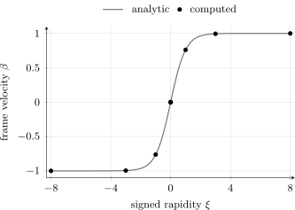
Signed rapidity and frame velocity. The solid curve is $\beta=\tanh\xi$; points are the exported default fixtures. Equal rapidity increments cease to look like equal velocity increments near the light-speed limit. The nearly coincident points around zero also test the small-rapidity implementation.

To reproduce the figure, place the TikZ/PGFPlots source beside lorentz-transformations-rapidity.csv. With a TeX distribution containing standalone, TikZ, and PGFPlots:

latex notebook-lorentz-rapidity.tex
dvisvgm --no-fonts notebook-lorentz-rapidity.dvi

The source can also find the retained CSV when compiled from the repository root. Only the points use the exported data; the continuous line is the analytic benchmark.

Independent checks and precision limits

The suite separates several kinds of evidence.

• Exact Fraction arithmetic verifies 36 exact assertions on rational fixtures, including boosts, compositions, and massive/massless shell-derivative determinants.
• Float64 matrix and vector tests compare metric, scalar products, inverse, determinant, and time orientation across fixed and seeded cases.
• The measure experiment differentiates the transformed spatial momentum with a five-point stencil. Each displaced point is independently put back on shell; the routine does not use the analytic derivative $dE/dp_i$.
• The photon test compares subtraction of large boosted components with $e^{-\xi}$ using separate decimal arithmetic.

Representative default results are:

Diagnostic	Retained result
Scientific comparisons	1,297 passed
Largest absolute metric residual	$6.16\times10^{-10}$
Largest scaled metric residual	$3.85\times10^{-16}$
Largest relative shell-Jacobian error	$4.29\times10^{-10}$, against tolerance $2\times10^{-7}$
Photon energy at $\xi=40$	Decimal $4.2483542553\times10^{-18}$; naive float64 subtraction $0$

The scaled metric error divides by a quantity of the size of the matrix products. It tests consistency relative to those large terms, not relative accuracy of every small invariant or output component. At $\xi=40$, the physical photon energy is nonzero even though the direct float64 subtraction loses it entirely.

The Jacobian uses steps $h,h/2,h/4$, with a default base step proportional to $10^{-4}E$. Truncation and roundoff compete; smaller steps need not improve the result monotonically. For example, the tested --fd-step 1e-7 run fails the derivative tolerance through roundoff. These finite tests support the implementation. They are not a proof of the Lorentz-group identities or an error bound for all input vectors. They also do not test invariance of an independently imposed momentum cutoff.

Modification exercises

A wrong boost that still preserves the metric. In a separate copy, reverse the signs of the boost’s mixed entries. Which check must fail even if the metric test passes?

Solution

The rest-particle passive-sign fixture fails: the transformed spatial momentum becomes $+m\sinh\xi\,\mathbf n$ instead of the declared negative value. The altered matrix represents the opposite boost, so it can still preserve the metric and have determinant one.

Separate derivative error from matrix stress. Repeat the experiment with different --fd-step values while keeping the rapidity range fixed. What should be compared before claiming convergence?

Solution

Compare the same physical shell points, the three derivative steps within each run, the analytic energy ratio, and the finest-pair difference. Also inspect the absolute matrix errors, which are not improved by changing the derivative step. At very small steps, roundoff can dominate and trigger a failed diagnostic rather than continued improvement.

Explain the lost photon energy. For a photon moving along the boost, rewrite $E'=\cosh\xi-\sinh\xi$ without subtracting two large nearly equal numbers.

Solution

For initial energy one, $E'=e^{-\xi}$. Computing this expression directly is stable over the demonstrated range, whereas subtracting the large hyperbolic functions can erase the small result. Stable light-cone variables or higher precision are useful when such small components matter.

References

• Rindler, Wolfgang. Introduction to Special Relativity. 2nd ed., Oxford University Press (1991). Finite boosts, rapidity, and invariant intervals.
• Weinberg, Steven. The Quantum Theory of Fields, Volume I: Foundations. Cambridge University Press (1995), sections 2.3 and 2.5. doi:10.1017/CBO9781139644167. Lorentz transformations and invariant one-particle measures.