Propagator Visualization Notebook

Retarded, advanced, and Feynman kernels can invert the same differential operator while giving different responses to the same source. This notebook makes the boundary data visible for one spatial Fourier mode, verifies the delta-source normalization, and compares direct convolution with independent forced oscillator evolution. The general propagator derivation remains at Klein–Gordon Propagators.

Required background. Klein–Gordon Propagators fixes the inverse and correlator conventions; Retarded and Advanced Green Functions explains the boundary-value distinction. Helpful background. Propagators to Correlators connects the scalar source factors to quantum-field expectation values.

Run the investigation. The program and retained results below support the stated experiment. Follow Running an Experiment for environment and output-directory guidance. The recorded evidence applies to its stated parameters and environment.

Unit-source scalar mode kernels

Use $\hbar=c=1$, $m>0$, one fixed spatial momentum magnitude $p$, and $\omega=\sqrt{p^2+m^2}$. For $L=\partial_t^2+\omega^2$, all three exported kernels obey $Lg_X=\delta(t)$:

$$\begin{aligned} g_R(t)&=\theta(t)\frac{\sin\omega t}{\omega},\\ g_A(t)&=-\theta(-t)\frac{\sin\omega t}{\omega},\\ g_F(t)&=\frac{i}{2\omega}e^{-i\omega|t|}. \end{aligned}$$

Each is continuous at zero and has $g_X'(0^+)-g_X'(0^-)=1$. The conventional scalar Feynman correlator in these conventions is instead $D_F=-ig_F$, with $LD_F=-i\delta$. The plotted $g_F$ is therefore a unit-source inverse, not a correlator with its factor of $-i$ silently omitted.

The code checks one-sided slopes and the integrated source equation

$$\begin{aligned} &g_X'(a)-g_X'(-a)\\ &\quad+\omega^2\int_{-a}^{a}g_X(t)\,dt=1, \qquad a>0. \end{aligned}$$

Away from zero, finite differences test the homogeneous equation. No ordinary pointwise derivative is used to represent the delta source. The source_jump column in the kernel CSV states the declared normalization; the measured jump and integrated residual checks are recorded separately in the JSON.

Compact-source responses and homogeneous data

For source half-width $T$, use the smooth compact bump

$$J(t)= \begin{cases} \exp\!\left(1-\dfrac{1}{1-(t/T)^2}\right), & |t|<T,\\ 0,& |t|\ge T. \end{cases}$$

Its peak amplitude is one in the chosen source units. The responses are

$$\phi_X(t)=\int_{-T}^{T}g_X(t-t')J(t')\,dt'.$$

Direct Simpson quadrature splits the integration interval at $t'=t$ whenever that point lies inside the source. This respects the kernel’s derivative change instead of applying a smooth quadrature assumption across it.

An independent fourth-order Runge–Kutta solver integrates $L\phi=J$ with zero past data for the retarded solution, or zero future data and backward time steps for the advanced solution. For the Feynman comparison, use

$$\begin{aligned} \phi_F(t)-\phi_R(t) &=\frac{i e^{i\omega t}}{2\omega} \widetilde J(\omega),\\ \widetilde J(\omega) &=\int_{-T}^{T}e^{-i\omega t'}J(t')\,dt'. \end{aligned}$$

This difference solves the homogeneous mode equation. Adding it to the retarded ODE solution supplies the Feynman boundary data independently of the direct Feynman convolution.

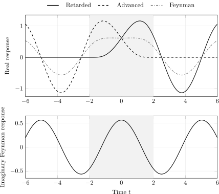
Default $m=1$, $p=0.75$, hence $\omega=1.25$, with source half-width $T=2$. The shaded interval is the source support. Retarded response vanishes before it, advanced response after it. The Feynman response has different homogeneous boundary data; its pre-source value is not a classical retarded signal. Times are in the inverse energy unit used for $m,p$; amplitudes use the declared source normalization.

In this even, real source example, the real Feynman curve is one half the sum of the retarded and advanced curves. Its imaginary part is a homogeneous oscillation. The plot contains only one spatial Fourier mode. It is not a spacetime light-cone plot and does not test full microcausality. No particle probability is assigned to the magnitude of these responses.

Separate numerical refinements

Four resolution questions appear in the exported results:

Study	What changes	What is being checked
Source quadrature	Simpson panel count	Convolution accuracy with fixed output times
Independent ODE evolution	RK4 time step	Accuracy of the separately evolved boundary solution
Off-source derivative	Centered-difference spacing	The homogeneous differential equation away from the impulse
Finite Feynman regulator	$\epsilon$	Approach of a different regulated inverse to its limiting prescription

The first three are different numerical tests. The last changes the operator. The 121 plotted output times merely sample the curves and are not any of those convergence parameters.

The fixed source-refinement fixture uses $\omega=1.3$, whereas the default configured figure uses $\omega=1.25$. Its final Simpson orders are approximately 4.00373, 4.00158, and 4.00500 for retarded, advanced, and Feynman responses. The independent RK4 order is approximately 4.00370. The centered second derivative has its expected second-order behavior away from the source.

For the default configured curves, the maximum difference between convolution and the independent ODE-based comparison is approximately $3.65\times10^{-9}$. This agreement concerns the stated source, window, and resolutions. A custom run must inspect its own response errors; passing the fixed fixtures does not certify every user-selected resolution.

Finite epsilon changes the inverse

With $\epsilon>0$ in energy-squared units, define

$$\begin{aligned} \Omega_\epsilon&=\sqrt{\omega^2-i\epsilon},\\ \operatorname{Re}\Omega_\epsilon&>0,\qquad \operatorname{Im}\Omega_\epsilon<0,\\ g_{F,\epsilon}(t) &=\frac{i}{2\Omega_\epsilon} e^{-i\Omega_\epsilon|t|}. \end{aligned}$$

It obeys $(L-i\epsilon)g_{F,\epsilon}=\delta$. Consequently, off the source,

$$Lg_{F,\epsilon}=i\epsilon g_{F,\epsilon}.$$

A nonzero residual of the unregularized operator is therefore expected. The regularization CSV exports that residual and the difference from $g_F$; ordinary off-source residual cells at $t=0$ remain empty. The regulator study compares decreasing $\epsilon$ on fixed sampled times and checks the decaying square-root branch. It does not establish uniform convergence on the entire infinite time axis.

Execute and reproduce the comparison

Download the standalone Python program. The retained run used Python 3.12.14 and NumPy 2.3.5 and passed 125 checks.

python -m pip install numpy==2.3.5
python propagator-visualization.py --output-dir propagator-results

Existing outputs are protected. Defaults include 512 Simpson panels per smooth segment, 960 ODE steps on $[-6,6]$, 121 output samples, and $\epsilon=0.05$ for the regulated table. For a finer independent ODE comparison, keep the panel count fixed:

python propagator-visualization.py --ode-steps 1920 --output-dir propagator-finer-ode

Download	Contents
Kernels CSV	Real and imaginary mode kernels and declared unit-source normalization
Responses CSV	Source, convolution, independent ODE comparison, and boundary-data labels
Refinement CSV	Separately labeled quadrature, ODE, derivative, and regulator studies
Regularization CSV	Configured finite-epsilon kernel and the required unregularized residual
JSON report	Checks, source and numerical parameters, conventions, environment, and hashes

The public JSON uses download paths; numerical results and CSV bytes retain the executed run’s values. Kernel and response rows are interleaved by time: retarded, advanced, Feynman at each time, rather than three contiguous blocks. Select kind before joining points into a curve.

Put the default responses CSV beside the TikZ source and use PGFPlots 1.18:

latex notebook-propagator-responses.tex
dvisvgm --no-fonts notebook-propagator-responses.dvi

The source selects each of the three interleaved sequences explicitly. Update its default 121-time selection if changing the output sample count.

Exercises

Two responses, one source. Subtract the retarded response from the Feynman response and apply $L$. Why does a nonzero pre-source difference not contradict the retarded boundary condition?

Solution

Both source terms cancel, leaving $L(\phi_F-\phi_R)=0$. The displayed difference is proportional to $e^{i\omega t}$ and solves that homogeneous equation. Only $\phi_R$ was required to vanish before the source. The other solution has different boundary data and is not a causal signal produced from those same zero past data.

A nonzero residual by design. Given $(L-i\epsilon)g_\epsilon=\delta$, derive the off-source residual of $L$. What would be wrong with demanding that this residual vanish at fixed nonzero $\epsilon$?

Solution

Away from the impulse, $Lg_\epsilon=i\epsilon g_\epsilon$. Requiring zero would impose the wrong differential operator. First verify the regulated identity and source jump; then study its $\epsilon\to0$ limit at the specified times.

More points, same accuracy. Why does doubling the plotted output samples alone not establish more accurate convolution or ODE evolution?

Solution

It requests more values from the same numerical procedure. The integration panel count and ODE step control those errors independently. Refine each while holding the physical source and an appropriate comparison set of times fixed; use the reported errors and observed orders to assess convergence.

References

• Schwartz, Matthew D. Quantum Field Theory and the Standard Model. Cambridge University Press, 2014. doi:10.1017/9781139540940.
• Tong, David. Quantum Field Theory. University of Cambridge lecture notes, 2006, sections 2.6–2.7. Free fields and propagators.