Klein Paradox

On the negative-energy branch of a Dirac step problem, an outgoing wave can have negative momentum. Choosing it by momentum sign alone changes the boundary condition and can produce a misleading flux interpretation. This notebook solves the two-component matching problem with incidence from the left, classifies channels by current, and sweeps the step through the positive continuum, evanescent gap, and negative continuum. The interpretation is developed at Klein Paradox.

Required background. Klein Paradox specifies the boundary-value problem; Dirac Current specifies its density and flux. Helpful background. Pair Creation explains why these stationary one-body coefficients alone are not a particle count.

Run the investigation. The program and retained results below support the stated experiment. Follow Running an Experiment for environment and output-directory guidance. The recorded evidence applies to its stated parameters and environment.

Stationary modes and outgoing current

Use $\hbar=c=1$, normal incidence in one fixed spin channel, and

$$H=-i\sigma_x\partial_x+m\sigma_z+V(x).$$

Here $V$ is potential energy, with $V_L$ on the left and $V_R$ on the right. Assume total energy $E$ with $E-V_L>m$, and no incident wave from the right. In a constant region, a spinor $w e^{ikx}$ satisfies

$$(k\sigma_x+m\sigma_z)w=\varepsilon w, \qquad \varepsilon=E-V.$$

For real propagating modes, $\varepsilon^2=k^2+m^2$ and

$$\rho=w^\dagger w,\qquad j=w^\dagger\sigma_xw,\qquad \frac j\rho=\frac k\varepsilon.$$

Thus outgoing on the right means $k/\varepsilon_R>0$. When $\varepsilon_R<-m$, it requires $k<0$. The program uses stable spinor charts on the two sides of the mass gap, avoiding a division by the small combination $\varepsilon+m$ near the negative threshold.

Real channel spinors are normalized to unit absolute current. With an incoming left mode $w_{\rm in}$, reflected mode $w_{\rm ref}$, and outgoing right mode $w_{\rm out}$, continuity at the step gives

$$w_{\rm in}+r w_{\rm ref}=\tau w_{\rm out}.$$

The algorithm solves this $2\times2$ linear system. In propagating regions, $R=|r|^2$ and $T=|\tau|^2$, and direct current evaluation checks $R+T=1$. For the owner’s exact example, $m=1$, $E=5/3$, $V_L=0$, $V_R=35/12$, the outgoing right momentum is $-3/4$, and

$$R=\frac{25}{49},\qquad T=\frac{24}{49}.$$

These are positive Dirac probability-current fractions with the stated one-sided incidence. They are not the signed Klein–Gordon charge current coefficients, nor vacuum pair-production probabilities.

Evanescent modes and excluded thresholds

For $|\varepsilon_R|<m$, choose $k=i\kappa$ with $\kappa>0$, so the right wave decays as $x\to+\infty$. Its current is zero. The program normalizes this mode to unit density at the interface; its nonzero coefficient $\tau$ is therefore not a unit-flux transmission amplitude. The transmitted flux remains $T=0$ and $R=1$.

At $\varepsilon_R=\pm m$, the propagating channel has zero current and cannot be normalized to unit flux. The sweep records these thresholds as excluded rows with empty $R,T$ entries. Empty values must not be replaced by zero measurements. For $m>0$, the adjacent limits are $R\to1$, $T\to0$; those limits do not construct a unit-flux mode at the threshold.

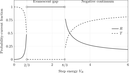
Default $E=5/3$, $m=1$, $V_L=0$ sweep. The right-channel thresholds are $V_R=2/3$ and $8/3$. Curves connect the retained uniform samples separately in each region; sampling is coarse close to the square-root thresholds. Hollow points show the analytic limits, while the channels at the exact thresholds remain excluded from the data.

The excluded points concern this asymptotic normalization. They do not declare a gap in the spectrum of the entire step Hamiltonian. The default profile download samples three analytic stationary solutions: a positive-continuum step, an evanescent step, and the negative-continuum example above. Increasing the profile sample count improves the plotted sampling; it does not change the matching calculation.

Independent checks and limiting regimes

The calculation checks the matching solution against closed amplitudes, direct currents, Hermitian eigensolver projectors, exact rational fixtures, and the unitary two-port scattering matrix where both channels propagate. In the default sweep the largest flux-balance discrepancy is approximately $4.44\times10^{-16}$. The condition number of each matching matrix is also exported; flux balance alone is not an accuracy estimate for every amplitude near a threshold.

Two fixed studies supplement the configured sweep. The threshold approach table uses $E=2$, $m=1$, so its threshold step energies are 1 and 3, rather than the default sweep’s $2/3$ and $8/3$. Its approaching propagating channels have $T\to0$. The derivative table likewise uses $E=2$, $m=1$, with steps $0.5$, $2$, and $3.3$. At points $x=\pm1.3$, away from the interface, centered differences test the stationary Dirac equation as the spacing decreases from $0.08$ to $0.01$.

The resulting residual divided by the spinor norm falls at second order. It still has energy units in natural units; it is not a universal dimensionless relative error. This finite-difference diagnostic does not mean that a mesh evolution produced the solution. At the discontinuity the spinor is continuous, but its derivative need not be.

The limiting-case table includes exact massless transmission for the tested nonthreshold steps and a massive nonrelativistic comparison. In the latter, hold physical mass $m=1$, incident kinetic energy $0.2$, and step energy $0.1$ fixed while increasing $c$. The solver’s mass slot then contains the rest energy $mc^2$, since its two-component equations use natural-unit form. This is a change of the relativistic scale, not a varying physical mass. The reflection approaches the Schrödinger result at order $c^{-2}$. In this scaling comparison the solver’s $k$ represents $c$ times physical momentum; the common velocity factor cancels from the flux ratios being compared.

The experiment assumes an abrupt stationary external step. It does not include a smooth interface, transverse momentum, a finite barrier, source recoil, radiation, switching history, or backreaction. Quantized in/out modes and an initial state are required for a pair-production calculation.

Run, inspect, and reproduce

Download the standalone Python program. The retained run used Python 3.12.14 and NumPy 2.3.5 and passed 4,007 checks. Use a fresh output directory:

python -m pip install numpy==2.3.5
python klein-paradox.py --output-dir klein-results

Existing output files are protected. The default step sweep has 121 uniform samples from zero to six plus two explicit excluded thresholds. For a finer sampled sweep:

python klein-paradox.py --samples 1201 --output-dir klein-finer-sweep

Download	Contents
Sweep CSV	Region, momentum, current, amplitudes, normalization, flux fractions, and conditioning
Profiles CSV	Analytically sampled spinor, density, and current for three representative steps
Thresholds CSV	Fixed $E=2,m=1$ approaches to the channel thresholds
Derivatives CSV	Fixed-fixture stationary-equation residuals versus finite-difference spacing
Limits CSV	Massless, large-step, and nonrelativistic comparisons
JSON report	Parameters, checks, excluded rows, environment, limitations, and file hashes

The public JSON replaces local output paths with download paths; numerical results and CSV bytes retain the executed run’s values. To reproduce the figure, put the default sweep CSV beside the TikZ source and use PGFPlots 1.18:

latex notebook-klein-flux.tex
dvisvgm --no-fonts notebook-klein-flux.dvi

The source selects the three default row blocks and adds hollow analytic threshold limits. Update the block selection and threshold positions when changing the sweep.

Exercises

Zero flux with nonzero amplitude. Inspect the right half of the evanescent profile. Why does a nonzero density there not imply nonzero transmission through the semi-infinite region?

Solution

The decaying mode has nonzero density but zero conserved current. Its coefficient measures interface amplitude in a unit-density normalization. Transmission is defined from outgoing asymptotic current, which vanishes. A finite barrier with a second interface would be a different matching problem.

Shift the energy origin. Use the importable match_step function to add the same constant to $E,V_L,V_R$. What should happen to the flux fractions? Why is shifting only $E,V_R$ in a zero-left-potential run a different operation?

Solution

Shifting all three leaves both kinetic energies $E-V_L$ and $E-V_R$ unchanged. The channel spinors and $R,T$ are therefore unchanged. If $V_L$ stays zero while $E$ changes, the incident kinetic energy and its spinor change, so the experiment is different.

Reverse the Klein-region momentum. At $\varepsilon_R<0$, replace the selected negative $k$ by positive $k$. Is the new mode still outgoing on the right?

Solution

No. Its velocity and current have the sign of $k/\varepsilon_R<0$. It travels toward the interface from the right. Matching it describes another boundary condition, not the same scattering solution with an anomalous probability.

References

• Calogeracos, Alex, and Norman Dombey. “History and physics of the Klein paradox.” Contemporary Physics 40, 313–321 (1999). doi:10.1080/001075199181387; arXiv:quant-ph/9905076.
• Gavrilov, S. P., and D. M. Gitman. “Quantization of charged fields in the presence of critical potential steps.” Physical Review D 93, 045002 (2016). doi:10.1103/PhysRevD.93.045002; arXiv:1506.01156.