Foldy–Wouthuysen Expansion

The static Foldy–Wouthuysen expansion can fail through an operator-ordering mistake even when its free-particle limit is correct. This notebook tests the ordered coefficients, evaluates their electromagnetic identities on exact polynomial fixtures, and measures the remaining odd terms using independently evaluated matrix exponentials. It also checks a scalar remainder bound for the pure-magnetic square root. The derivation and physical approximation conditions remain at Foldy–Wouthuysen Expansion.

Required background. Foldy–Wouthuysen Expansion fixes the terms and power counting; Foldy–Wouthuysen Transformation fixes the representation change. Helpful background. Minimal Coupling supplies the signed-charge commutators.

Run the investigation. The program and retained results below support the stated experiment. Follow Running an Experiment for environment and output-directory guidance. The recorded evidence applies to its stated parameters and environment.

Ordered static Hamiltonian

Retain $c$ and $\hbar$, take $m>0$, and hold the smooth static potentials, charge, and spatial derivatives fixed in the inverse-$c$ expansion. Define

$$\begin{aligned} H&=\beta mc^2+cD+V,\\ D&=\boldsymbol\alpha\cdot\boldsymbol\pi,\qquad V=q\Phi,\\ \boldsymbol\pi&=-i\hbar\nabla-q\mathbf A. \end{aligned}$$

The exact word algebra imposes only $\beta^2=I$, $\beta D=-D\beta$, and $\beta V=V\beta$. In particular, it never replaces $DV$ by $VD$. With $\psi_{\rm FW}=U\psi$, the retained even Hamiltonian is

$$\begin{aligned} H_{\rm even}^{(2)} ={}&\beta mc^2+V+\frac{\beta D^2}{2m}\\ &-\frac{\beta D^4}{8m^3c^2} -\frac{[D,[D,V]]}{8m^2c^2}. \end{aligned}$$

The coefficient CSV encodes an ordered term as its rational coefficient, power of $\lambda=1/c$, power of $m$, and word in B, D, and V. Here B denotes $\beta$, not a magnetic field. For example, DV and VD are distinct records in the second generator.

The code labels its successive anti-Hermitian generators $G_1,G_2,G_3$, beginning with $G_1=\beta D/(2mc)$. Exact BCH arithmetic shows that the residual odd terms after the first and second stages begin at $c^{-1}$ and $c^{-3}$ respectively. The third stage removes the latter before assigning a formal full-Hamiltonian remainder of $O(c^{-4})$. Merely verifying the displayed even terms does not verify that the odd remainder has been removed to the same accuracy.

Independent electromagnetic and matrix checks

The polynomial differential-operator fixtures check the ordered square

$$F=D^2=\boldsymbol\pi^2-q\hbar\boldsymbol\Sigma\cdot\mathbf B$$

and its full square:

$$\begin{aligned} F^2={}&(\boldsymbol\pi^2)^2\\ &-q\hbar\{ \boldsymbol\pi^2,\boldsymbol\Sigma\cdot\mathbf B\}\\ &+q^2\hbar^2\mathbf B^2. \end{aligned}$$

The braces are an anticommutator of operators, including the derivatives acting on a nonuniform magnetic field. The electric comparison is

$$\begin{aligned} [D,[D,V]] ={}&q\hbar^2\nabla\cdot\mathbf E\\ &+q\hbar\boldsymbol\Sigma\cdot (\mathbf E\times\boldsymbol\pi -\boldsymbol\pi\times\mathbf E). \end{aligned}$$

Five static backgrounds, three charges $q=-2,0,2$, and three complex polynomial spinor fixtures give 225 exact field identity checks. These fixtures set $\hbar=2$, so they test its powers explicitly. Dropping the magnetic terms from $F^2$ is detected in eighteen cases. Polynomial fixtures test local differential identities; they are not normalizable wave functions or spectral calculations.

For a separate finite $4\times4$ fixture, the program diagonalizes the Hermitian matrix $iG_j$ to evaluate each exponential. It then computes

$$\begin{aligned} H_j&=e^{G_j}H_{j-1}e^{-G_j},\\ (H_j)_{\rm odd}&=\frac{H_j-\beta H_j\beta}{2}. \end{aligned}$$

This numerical transformation does not use the truncated BCH series as its exponential. The matrices obey the even-odd grading and have $[D,V]\ne0$; they are an algebra fixture, not a spatial electromagnetic solver. All residual norms in this table and figure are Frobenius norms, in the fixed numerical units of that fixture.

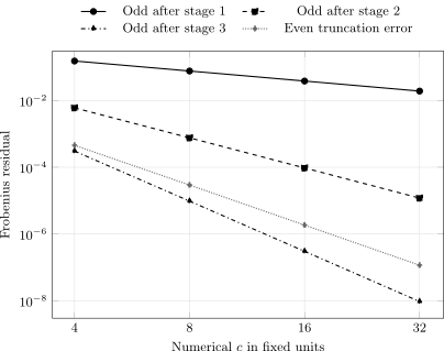
Default matrix study with $m=1$. The odd residual after each successive transformation and the even-part truncation error are computed from the retained CSV. Connecting segments guide the eye between four sampled values; they do not represent a continuum convergence proof.

For an error $\varepsilon(c)$, the exported observed order is $\log_2[\varepsilon(c)/\varepsilon(2c)]$. Between $c=16$ and $32$, the default values are:

Residual	Expected inverse power	Observed order
Odd part after stage 1	1	0.99962
Odd part after stage 2	3	2.99913
Odd part after stage 3	5	4.99884
Even-part truncation error	4	3.99702

Custom matrix parameters append a configured_diagnostic study to the fixed fixed_self_check records. Inspect the study column before comparing or plotting rows. Passing the fixed checks does not guarantee that arbitrary parameter choices are in their asymptotic regime.

Magnetic square-root remainder

For a nonnegative spectral value of $F$, put $r=F/(m^2c^2)$ in the scalar comparison. The dimensionless remainder

$$R(r)=\sqrt{1+r}-1-\frac r2+\frac{r^2}{8}$$

obeys

$$\frac{r^3}{16(1+r)^{5/2}} \le R(r)\le\frac{r^3}{16}, \qquad r\ge0.$$

The program uses 160-digit decimal arithmetic by default, including $r=10^{-30}$, where ordinary double-precision subtraction would lose the remainder. Its eleven values range from zero to $10^4$. The bounds hold throughout that range, but a low-energy truncation need not be useful when $r$ is large. Multiply the dimensionless remainder by $mc^2$ to obtain the positive energy-branch error.

A uniform operator bound follows only after restricting to a bounded spectral interval. Neither this scalar sweep nor the finite matrix norms establishes an operator-norm expansion for unbounded momentum. Time-dependent potentials also require the extra $i\hbar\dot U U^\dagger$ term; they are outside this static calculation.

Reproduce the calculation and figure

The standalone Python program was executed with Python 3.12.14 and NumPy 2.3.5. The default run passes 280 checks. Download it and run in a fresh output directory:

python -m pip install numpy==2.3.5
python foldy-wouthuysen-expansion.py --output-dir fw-results

The program protects existing outputs. For a different finite-matrix diagnostic, use, for example:

python foldy-wouthuysen-expansion.py --mass 2 --first-c 2 --output-dir fw-mass-two

Download	Contents
Coefficients CSV	Exact rational ordered words for the Hamiltonian, generators, remainder, and retained even terms
Fields CSV	Background, charge, Planck constant, spinor fixture, identity, and verdict
Matrices CSV	Residuals and observed orders for successive numerical transformations
Roots CSV	Decimal square roots, dimensionless remainders, and bounds
JSON report	Individual checks, parameters, environment, limitations, and source/output hashes

Public report paths point to these downloads; the computed values and CSV bytes retain the executed run’s values. To recreate the figure, place the default matrices CSV beside the TikZ source and use a TeX installation with PGFPlots 1.18:

latex notebook-fw-orders.tex
dvisvgm --no-fonts notebook-fw-orders.dvi

Exercises

The missing odd term. A calculation verifies the even Hamiltonian through $c^{-2}$ after two transformations. Why can its full residual still scale as $c^{-3}$?

Solution

Even projection discards the odd part. The second transformation removes the $c^{-1}$ odd term but leaves a generic $c^{-3}$ odd remainder. It therefore dominates the $c^{-4}$ even error unless removed by the next generator. The two residuals answer different questions.

Magnetic ordering. Expand $F^2$ with $F=P-Q$, where $P=\boldsymbol\pi^2$ and $Q=q\hbar\boldsymbol\Sigma\cdot\mathbf B$. Why is replacing the cross terms by $-2PQ$ not generally allowed?

Solution

The expansion is $P^2-PQ-QP+Q^2$. For a nonuniform field, derivatives inside $P$ act on $\mathbf B$ as well as on the spinor, and $[P,Q]$ need not vanish. The anticommutator retains both actions. Even for a uniform field, deleting $Q^2$ needs an additional approximation beyond the stated fixed-field inverse-$c$ counting.

A bound that is too loose. Evaluate the quadratic square-root approximation at $r=10$ and compare its sign with the exact answer. Does a valid remainder bound make the approximation useful there?

Solution

The approximation is $1+5-100/8=-6.5$, whereas the exact value is $\sqrt{11}>0$. The positive remainder still satisfies the stated bounds. Those bounds certify an error interval, not a small relative error outside the low-$r$ regime.

References

• Bjorken, James D., and Sidney D. Drell. Relativistic Quantum Mechanics. McGraw–Hill, 1964.
• Foldy, Leslie L., and Siegfried A. Wouthuysen. “On the Dirac Theory of Spin 1/2 Particles and Its Non-Relativistic Limit.” Physical Review 78, 29–36 (1950). doi:10.1103/PhysRev.78.29.