Variational Helium Notebook

This notebook asks how far one optimized orbital exponent can take the helium ground state, and makes every comparison use the same Hamiltonian. The calculation is analytically solvable, but it is still a useful computational benchmark because it distinguishes:

• a different, noninteracting Hamiltonian from a trial state for full helium;
• an unoptimized product from its variational optimum;
• energy accuracy from parameter and wavefunction accuracy;
• single-orbital restriction from electron correlation;
• and printed digits from validated digits.

For a point nucleus of charge $Z=2$ and infinite nuclear mass, the retained program finds

$$\zeta_*=\frac{27}{16}=1.6875$$

and

$$E(\zeta_*) = -\frac{729}{256}E_{\mathrm h} = -2.847\,656\,25E_{\mathrm h}.$$

This is a strict variational upper bound for the stated nonrelativistic Hamiltonian, but it remains

$$0.056\,068\,127\,034\,119E_{\mathrm h}$$

above a high-precision nonrelativistic clamped-nucleus reference. The gap is not all “correlation energy”: part comes from restricting the Hartree–Fock orbital itself to a one-parameter exponential.

Run the investigation. The program and retained results below support the stated experiment. Follow Running an Experiment for environment and output-directory guidance. The recorded evidence applies to its stated parameters and environment.

Canonical Scope

The complete analytic evaluation of the Coulomb integral and the effective charge derivation belong to Variational Estimate for the Helium Atom. The Helium Atom page owns helium’s spectrum, singlet–triplet structure, precision hierarchy, and role as an atomic benchmark. The Variational Principle owns the upper-bound theorem.

This page owns the reproducible notebook experiment:

• encode the analytic energy decomposition;
• separate two independent-particle baselines;
• optimize $\zeta$ analytically and numerically;
• compare machine-readable results with retained references;
• verify upper-bound and virial statements;
• expose optimizer conditioning at a stationary energy;
• audit units and ionization conventions;
• and identify which missing physics contributes to the remaining deficit.

It does not duplicate the full six-dimensional integral derivation or present the retained literature references as outputs of the notebook.

Reproducibility Contract

Item	Notebook choice
system	neutral helium, $Z=2$, two electrons
Hamiltonian	nonrelativistic Coulomb, infinite-mass point nucleus
state	spatially symmetric $1s^2$ singlet ground-state trial
trial family	two identical hydrogenic $1s$ orbitals with exponent $\zeta>0$
target	total electronic energy and its components
optimizer	analytic stationary point plus bracketed golden-section search
arithmetic	IEEE 754 binary64 through Python float
dependencies	Python 3 standard library only
randomness	none
validation	analytic agreement, upper bound, virial stationarity, finite-difference gradient, ordering
artifacts	program, energy-curve CSV, summary CSV, metadata JSON

The numerical minimizer is intentionally redundant. It does not make the analytic problem more accurate; it tests the encoded objective and illustrates how a general optimizer behaves near a variational stationary point.

Hamiltonian and Units

In Hartree atomic units,

$$\hbar=m_e=e=4\pi\epsilon_0=1.$$

The clamped-nucleus electronic Hamiltonian is

$$H = -\frac12\nabla_1^2 -\frac12\nabla_2^2 -\frac{Z}{r_1} -\frac{Z}{r_2} +\frac{1}{r_{12}},$$

where

$$r_{12}=|\mathbf r_1-\mathbf r_2|.$$

Distances are measured in Bohr radii $a_0$ and energies in Hartree $E_{\mathrm h}$. The zero is a bare nucleus plus two electrons at rest at infinite separation.

What the exponent means dimensionally

The normalized orbital is written in atomic-unit coordinates as

$$\phi_\zeta(\mathbf r) = \left( \frac{\zeta^3}{\pi} \right)^{1/2} e^{-\zeta r}.$$

Here the numerical coordinate $r$ is measured in $a_0$, so $\zeta$ is numerically an inverse-Bohr scale. Restoring dimensions,

$$\phi_\zeta(\mathbf r) = \left[ \frac{(\zeta/a_0)^3}{\pi} \right]^{1/2} \exp\left(-\frac{\zeta r}{a_0}\right).$$

The dimensionless number $\zeta$ can also be interpreted as an effective nuclear charge for this hydrogenic shape. It is not a measured nuclear charge and need not be an integer.

Unit audit

Quantity	Atomic-unit dimension	Notebook value
$r$	$a_0$	input coordinate
$\zeta$	$a_0^{-1}$ numerically	optimized as a dimensionless exponent
kinetic expectation	$E_{\mathrm h}$	$\zeta^2$
Coulomb expectations	$E_{\mathrm h}$	linear in $\zeta$
total energy	$E_{\mathrm h}$	sum of components
ionization energy	$E_{\mathrm h}$	difference of two total energies

Convert to electronvolts or inverse centimetres only after the Hartree result is established, using a stated constants release. Rounding a conversion factor early can obscure whether a discrepancy is numerical or metrological.

Baseline 1: Turn Off Repulsion

If the electron–electron interaction is removed, the Hamiltonian becomes

$$H_0 = \sum_{i=1}^{2} \left( -\frac12\nabla_i^2-\frac{Z}{r_i} \right).$$

Each electron occupies an exact hydrogenic $1s$ orbital with exponent $\zeta=Z$, so

$$E_0=-Z^2.$$

For helium,

$$E_0=-4E_{\mathrm h}.$$

This is an exact result for $H_0$, but not a variational estimate for the full Hamiltonian $H$. It lies below the exact helium energy because a positive interaction was deleted. The variational theorem compares trial states for one fixed Hamiltonian; it does not order different Hamiltonians.

This baseline answers a physical question: how large is the direct effect of electron repulsion relative to two independent Coulomb electrons? It cannot be inserted into the full-Hamiltonian upper-bound ladder.

Baseline 2: Bare Exponent in the Full Hamiltonian

Keep $\zeta=Z$, but now evaluate the full $H$, including $1/r_{12}$. For $Z=2$,

$$\begin{aligned} \langle T\rangle &=4,\\ \langle V_{\mathrm{nuc}}\rangle &=-8,\\ \langle V_{ee}\rangle &=\frac54. \end{aligned}$$

Therefore

$$E(\zeta=2) = 4-8+\frac54 = -\frac{11}{4} = -2.75E_{\mathrm h}.$$

This is a valid variational upper bound for the full Hamiltonian. It uses an admissible normalized trial state but has not yet allowed the orbital to expand in response to screening.

Keeping these two baselines separate prevents the common but severe mistake of calling $-4E_{\mathrm h}$ a variational helium energy.

Trial State and Fermionic Symmetry

Use the spatial product

$$\Phi_\zeta(\mathbf r_1,\mathbf r_2) = \phi_\zeta(\mathbf r_1) \phi_\zeta(\mathbf r_2).$$

It is symmetric under exchange of spatial coordinates. The full two-electron state is antisymmetric because it is multiplied by the spin singlet

$$\chi_{00} = \frac{ |\uparrow\downarrow\rangle -|\downarrow\uparrow\rangle }{ \sqrt2 }.$$

Thus

$$\Psi_\zeta = \Phi_\zeta\chi_{00}$$

is a legal fermionic trial state for the helium ground-state symmetry.

Equivalently, it is the Slater determinant formed from $\phi_\zeta\alpha$ and $\phi_\zeta\beta$. For helium, the one-parameter family can therefore be viewed as a severely constrained restricted Hartree–Fock family: the spatial orbital is forced to remain a pure hydrogenic exponential.

Energy Components

For the normalized trial state,

$$\begin{aligned} T(\zeta) &= \left\langle -\frac12\nabla_1^2-\frac12\nabla_2^2 \right\rangle =\zeta^2, \\ V_{\mathrm{nuc}}(\zeta) &= \left\langle -\frac{Z}{r_1}-\frac{Z}{r_2} \right\rangle =-2Z\zeta, \\ V_{ee}(\zeta) &= \left\langle \frac1{r_{12}} \right\rangle =\frac58\zeta. \end{aligned}$$

The total is

$$E(\zeta;Z) = \zeta^2-2Z\zeta+\frac58\zeta.$$

The $5\zeta/8$ integral is the only genuinely two-electron integral in this trial family. Its analytic derivation remains at the canonical worked example linked above.

Minimal executable cell

The retained program encodes the decomposition directly:

def energy_components(zeta: float, nuclear_charge: float = 2.0):
    kinetic = zeta * zeta
    nuclear = -2.0 * nuclear_charge * zeta
    repulsion = 5.0 * zeta / 8.0
    return kinetic, nuclear, repulsion

Keeping components separate supports unit checks, virial validation, and clear diagnosis of a sign error. An implementation that stores only the total can accidentally obtain a plausible minimum from compensating mistakes.

Analytic Optimization

Differentiate:

$$\frac{dE}{d\zeta} = 2\zeta-2Z+\frac58.$$

The stationary exponent is

$$\zeta_* = Z-\frac5{16}.$$

Because

$$\frac{d^2E}{d\zeta^2}=2>0,$$

this is the unique minimum for $\zeta>0$ whenever $Z>5/16$.

Completing the square gives

$$E(\zeta;Z) = \left( \zeta-Z+\frac5{16} \right)^2 - \left( Z-\frac5{16} \right)^2.$$

Hence

$$E_*(Z) = - \left( Z-\frac5{16} \right)^2.$$

For helium,

$$\begin{aligned} \zeta_* &= 2-\frac5{16} =\frac{27}{16}, \\ E_* &= -\left(\frac{27}{16}\right)^2 =-\frac{729}{256}E_{\mathrm h}. \end{aligned}$$

The screening parameter in this ansatz is

$$\sigma=Z-\zeta_*=\frac5{16}.$$

It is an optimized scale parameter, not a claim that one electron screens a fixed fraction of charge at every radius.

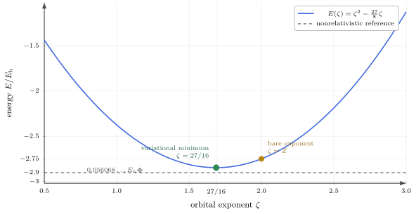
The full-Hamiltonian trial energy is a parabola. The optimized exponent lowers the bare-$Z$ trial from $-2.75E_{\mathrm h}$ to $-2.84765625E_{\mathrm h}$, but the entire one-parameter curve remains above the exact nonrelativistic clamped-nucleus energy. The noninteracting $-4E_{\mathrm h}$ result is absent because it belongs to a different Hamiltonian.

Numerical Experiment

The program performs two numerical tasks:

1. sample $E(\zeta)$ at 501 equally spaced points on $0.5\le\zeta\le3$ for the retained curve;
2. minimize the objective independently with a bracketed golden-section search.

The scan visualizes the landscape and confirms that the analytic optimum lies inside the bracket. The scan spacing does not determine the final minimum. The golden-section search retains a bracket and assumes only that the objective is unimodal on the interval.

Run:

python variational-helium.py --output-dir variational-helium-output

The retained run prints:

analytic zeta       = 1.687500000000000
numeric zeta        = 1.687499999849360
optimized energy    = -2.847656250000000 Eh
unoptimized energy  = -2.750000000000000 Eh
no-repulsion model  = -4.000000000000000 Eh
trial deficit       = 0.056068127034119 Eh
HF correlation gap  = 0.042044381422119 Eh
validation          = all checks passed

The no-repulsion value is printed with an explicit model label so that it cannot be mistaken for a full-Hamiltonian trial energy.

Why the numerical exponent is not exact

The energy can be written exactly as

$$E(\zeta) = E_* +(\zeta-\zeta_*)^2.$$

An exponent error $\delta\zeta$ therefore changes the energy only by

$$\delta E=(\delta\zeta)^2.$$

Near the minimum, binary64 energy evaluations cannot distinguish changes much smaller than roughly machine precision times the energy scale. An energy-only optimizer therefore loses parameter resolution at approximately the square root of the energy floor.

The retained search gives

$$|\zeta_{\mathrm{num}}-\zeta_*| \approx 1.51\times10^{-10},$$

while both energies round to the same binary64 value. This is not optimizer failure. It is a concrete instance of a general variational fact: stationary energies can look much more accurate than nonlinear parameters or wavefunctions.

The validation threshold reflects this conditioning:

• exponent agreement must be better than $5\times10^{-9}$;
• energy agreement must be better than $2\times10^{-13}E_{\mathrm h}$.

Demanding the same absolute tolerance for both would misrepresent the information contained in the objective.

Retained Results

For $\zeta=27/16$, the exact component values within the trial family are

$$\begin{aligned} T &= \frac{729}{256} =2.847\,656\,25, \\ V_{\mathrm{nuc}} &= -\frac{27}{4} =-6.75, \\ V_{ee} &= \frac{135}{128} =1.054\,687\,5, \\ V &= -\frac{729}{128} =-5.695\,312\,5, \\ E &= -\frac{729}{256} =-2.847\,656\,25. \end{aligned}$$

All energies in this display are in $E_{\mathrm h}$.

Model or state	Hamiltonian	Energy $E_{\mathrm h}$	Status
independent electrons, no $1/r_{12}$	$H_0$	$-4$	exact for a different Hamiltonian
product with $\zeta=Z=2$	full $H$	$-2.75$	valid unoptimized upper bound
product with $\zeta=27/16$	full $H$	$-2.84765625$	optimized one-parameter upper bound
Hartree–Fock limit	full $H$	approximately $-2.861679995612$	retained literature reference
nonrelativistic clamped-nucleus limit	full $H$	approximately $-2.903724377034119$	retained literature reference

The final two rows are not computed by this program. They are reference values used to interpret the trial family and are labeled as such in the summary CSV.

Variational ordering

For the same full Hamiltonian,

$$E_{\mathrm{exact}} \le E_{\mathrm{HF}} \le E_{\zeta_*} \le E_{\zeta=Z}.$$

Numerically,

$$-2.903724\ldots < -2.861680\ldots < -2.84765625 < -2.75.$$

Lower energy is better. The $-4E_{\mathrm h}$ no-repulsion value does not belong in this chain.

Virial Validation

For a Coulomb Hamiltonian and a scale-stationary trial state, the virial condition is

$$2T+V=0.$$

In this family,

$$\begin{aligned} 2T+V &= 2\zeta^2 -2Z\zeta +\frac58\zeta \\ &= \zeta \frac{dE}{d\zeta}. \end{aligned}$$

At $\zeta=\zeta_*$,

$$2T+V=0.$$

The retained analytic result satisfies this exactly in binary64 arithmetic:

$$2(2.84765625)-5.6953125=0.$$

At the unoptimized bare exponent,

$$2T+V = 8-8+\frac54 =\frac54,$$

so its nonzero virial residual correctly diagnoses unfinished scale optimization.

The virial check is independent of the known optimum but not independent of the encoded energy components. A sign mistake repeated in both the objective and residual could still pass; the exact benchmark values and component table provide additional checks.

Finite-Difference Gradient Check

The program evaluates

$$\left. \frac{dE}{d\zeta} \right|_{\zeta_*} \approx \frac{ E(\zeta_*+h)-E(\zeta_*-h) }{ 2h }$$

with

$$h=10^{-5}.$$

For this quadratic objective the centered formula is exact in symbolic arithmetic, and the retained binary64 value is zero. In a general notebook, vary $h$: a large step exposes truncation error while a very small step exposes cancellation.

This test would catch an optimizer that stopped away from stationarity even if its energy happened to round close to the reference value.

Upper-Bound Validation

The trial state is normalized, has the correct singlet fermionic symmetry, and belongs to the form domain of the nonrelativistic Coulomb Hamiltonian. Therefore

$$E(\zeta)\ge E_{\mathrm{exact}}$$

for every $\zeta>0$.

The program checks

$$-2.84765625 \ge -2.9037243770341196.$$

This comparison is useful as a regression test, but the theorem does not derive from the stored decimal. If a future run falls below the reference, at least one of the following has happened:

• the Hamiltonian changed;
• the trial expectation was evaluated incorrectly;
• the reference convention changed;
• numerical integration or normalization failed;
• or the output units were mislabeled.

Silently celebrating a lower “variational” energy would be the wrong response.

Ionization-Energy Check

For the same infinite-mass nonrelativistic convention, the one-electron helium ion has

$$E(\mathrm{He}^+)=-\frac{Z^2}{2}=-2E_{\mathrm h}.$$

The first ionization energy inferred from a neutral-helium approximation is

$$I_1 = E(\mathrm{He}^+)-E(\mathrm{He}).$$

The optimized trial gives

$$I_1^{(\zeta)} = -2-(-2.84765625) = 0.84765625E_{\mathrm h}.$$

The nonrelativistic reference gives

$$I_1^{(\mathrm{NR})} \approx 0.9037243770341196E_{\mathrm h}.$$

The equality of the ionization-energy deficit and total-energy deficit occurs because the one-electron ion is exact in this model. In a general comparison, errors in both charge states contribute and can cancel.

Do not compare the neutral total energy itself with an experimental ionization energy; they have different zeros and dimensions of interpretation even when both are quoted in Hartree.

What Screening Captures

The optimized orbital is more diffuse than the bare $Z=2$ hydrogenic orbital:

$$\zeta_*=1.6875<2.$$

Its mean radius is

$$\langle r\rangle = \frac{3}{2\zeta_*} = \frac89a_0 \approx0.8889a_0,$$

compared with

$$\frac34a_0$$

for $\zeta=2$. Variational optimization therefore captures an average expansion caused by electron repulsion.

It also balances kinetic, nuclear-attraction, and direct-repulsion energy rather than simply subtracting a guessed screening charge from $Z$.

What screening does not capture

The spatial probability factorizes:

$$|\Phi_\zeta(\mathbf r_1,\mathbf r_2)|^2 = |\phi_\zeta(\mathbf r_1)|^2 |\phi_\zeta(\mathbf r_2)|^2.$$

Conditional on one electron’s position, the other electron’s distribution does not move. The ansatz cannot create a correlation hole that favors large $r_{12}$.

For an opposite-spin electron pair, the exact Coulomb wavefunction satisfies the electron–electron cusp condition

$$\left. \frac{1}{\Psi} \frac{\partial\Psi}{\partial r_{12}} \right|_{r_{12}=0} = \frac12$$

in atomic units. The product state has no explicit $r_{12}$ dependence and gives zero for this derivative. Orbital screening improves the one-electron scale but cannot repair the two-electron cusp.

Decomposing the Remaining Deficit

Define the positive trial deficit

$$\Delta_{\mathrm{trial}} = E_{\zeta_*}-E_{\mathrm{exact}}.$$

Using the retained references,

$$\Delta_{\mathrm{trial}} \approx 0.056068127034119E_{\mathrm h}.$$

Insert the Hartree–Fock limit:

$$\begin{aligned} \Delta_{\mathrm{trial}} ={}& \left( E_{\zeta_*}-E_{\mathrm{HF}} \right) \\ &+ \left( E_{\mathrm{HF}}-E_{\mathrm{exact}} \right). \end{aligned}$$

The two positive pieces are approximately

$$E_{\zeta_*}-E_{\mathrm{HF}} = 0.014023745612E_{\mathrm h}$$

and

$$E_{\mathrm{HF}}-E_{\mathrm{exact}} = 0.042044381422119E_{\mathrm h}.$$

The first measures restriction of the self-consistent one-orbital shape to a single exponential. The second is the magnitude of the conventional nonrelativistic clamped-nucleus correlation energy:

$$E_{\mathrm c} = E_{\mathrm{exact}}-E_{\mathrm{HF}} \approx -0.042044381422119E_{\mathrm h}.$$

Calling the entire $0.0561E_{\mathrm h}$ gap “correlation energy” would conflate orbital-shape incompleteness with correlation beyond the Hartree–Fock determinant.

Large-Z Interpretation

For a helium-like ion of nuclear charge $Z$,

$$E_*(Z) = - \left( Z-\frac5{16} \right)^2 = -Z^2+\frac58Z-\frac{25}{256}.$$

The first two terms match the structure expected when electron repulsion is treated as a first-order correction to two hydrogenic electrons:

$$E(Z) = -Z^2+\frac58Z+O(Z^0).$$

The one-parameter optimization adds a particular constant term $-25/256$, but it does not reproduce the exact full $1/Z$ expansion. This explains why the ansatz becomes relatively better as $Z$ grows while remaining structurally incapable of exact correlation.

When changing $Z$ in the program, the retained helium Hartree–Fock and exact reference checks are disabled. Reusing helium reference numbers for another ion would be a model error, not a numerical one.

Downloadable Program and Data

• Download the Python program
• Download the energy-curve CSV
• Download the benchmark summary CSV
• Download the run metadata JSON

The program requires only Python’s standard library. Run it with:

python variational-helium.py --output-dir variational-helium-output

Optional arguments expose the nuclear charge, exponent interval, and curve resolution:

python variational-helium.py \
  --nuclear-charge 2 \
  --zeta-min 0.5 \
  --zeta-max 3.0 \
  --points 501 \
  --output-dir variational-helium-output

The source carries the SPDX identifier MIT; the program and generated data are released under the MIT License.

Artifact roles

Artifact	Purpose
program	authoritative executable formulas, optimizer, checks, and writers
energy-curve CSV	every sampled component and virial residual versus $\zeta$
summary CSV	model-separated baselines, optimized results, and retained references
metadata JSON	environment, parameters, validation outcomes, and output inventory

The summary deliberately includes a hamiltonian column and a variational_for_full_H field. These make it difficult for downstream plots to place the $-4E_{\mathrm h}$ noninteracting result in the full-helium variational ladder by accident.

Reproducibility Metadata

Item	Retained run
operating system	Windows 11, x86-64
Python	CPython 3.12.13
scalar type	IEEE 754 binary64
external packages	none
nuclear charge	$Z=2$
exponent scan	$0.5\le\zeta\le3.0$
curve points	501
optimizer	bracketed golden-section search
optimizer iterations	68
random seed	none; deterministic
analytic exponent error	exactly zero by construction
numerical exponent error	$1.5064\times10^{-10}$
numerical energy error	zero at binary64 resolution
license	MIT

The metadata JSON records the full platform string and all validation flags. For archival reruns, retain the console output and generated files together.

Validation Ledger

Claim	Check	Retained outcome
encoded objective matches derivation	compare analytic components at $\zeta_*$	exact rational values recovered
numerical optimizer finds same basin	golden-section result versus analytic $\zeta_*$	difference $1.51\times10^{-10}$
numerical energy reaches minimum	analytic versus numerical energy	equal in binary64
optimum is stationary	centered finite-difference gradient	zero in binary64
scale is optimized	analytic virial residual	zero
optimization helps	compare $\zeta_*$ with $\zeta=Z$	energy lowered by $0.09765625E_{\mathrm h}$
result remains variational	compare with nonrelativistic reference	upper bound passes
trial remains above HF	compare with HF-limit reference	ordering passes
outputs are deterministic	no random input and fixed formulas	repeatable

No one row is sufficient. The upper-bound comparison could pass despite a small algebraic error, while analytic agreement alone would not show that the program labels the no-repulsion model correctly.

What is not independently verified here

The notebook does not recompute:

• the analytic $5\zeta/8$ Coulomb integral by numerical quadrature;
• the Hartree–Fock limit;
• the high-precision nonrelativistic energy;
• finite-mass, relativistic, or QED corrections;
• experimental ionization energies.

Those are either canonical derivations or retained external references. A future numerical-integration extension should be validated against the analytic integral before it replaces any formula.

Error and Scope Ledger

The optimized value has essentially no numerical uncertainty at the displayed precision because the objective is analytic and one dimensional. Its physical error is dominated by the ansatz:

Source	Present?	Consequence
optimizer error	negligible for energy	exponent limited by stationary-point conditioning
arithmetic error	below displayed energy digits	visible in numerical exponent and component virial residual
one-orbital shape restriction	yes	about $0.0140E_{\mathrm h}$ relative to HF limit
correlation beyond one determinant	yes	about $0.0420E_{\mathrm h}$
finite nuclear mass	omitted	needed for isotope-specific comparison
relativity and QED	omitted	needed beyond the nonrelativistic model
nuclear size	omitted	negligible at this scale but conceptually separate
external reference uncertainty	not represented by printed decimals	consult source calculations

The word “exact” in the reference row means exact to the quoted numerical precision for the nonrelativistic clamped-nucleus Coulomb Hamiltonian. It does not mean exact physical helium.

Extensions

Numerical Coulomb integral

Replace

$$V_{ee}=\frac58\zeta$$

by a verified radial quadrature. For a spherical one-electron density $\rho_\zeta(r)$, angular averaging gives

$$\left\langle\frac1{r_{12}}\right\rangle = \int_0^\infty\!\!\int_0^\infty \frac{ 4\pi r_1^2\rho_\zeta(r_1) \,4\pi r_2^2\rho_\zeta(r_2) }{ \max(r_1,r_2) } \,dr_1\,dr_2.$$

Converge domain, radial quadrature, and singular diagonal treatment separately. Recovery of $5\zeta/8$ is then an implementation benchmark.

Flexible self-consistent orbital

Expand the common spatial orbital in a radial basis and optimize its coefficients. This approaches the helium restricted Hartree–Fock limit and isolates the $0.0140E_{\mathrm h}$ one-orbital-shape deficit. The later Hartree–Fock notebook owns that nonlinear workflow.

Two orbital exponents

A symmetric form such as

$$\Phi_{\alpha\beta} \propto e^{-\alpha r_1-\beta r_2} + e^{-\beta r_1-\alpha r_2}$$

allows one electron to be compact while the other is diffuse without assigning permanent identities. It can improve radial correlation but still has no general explicit $r_{12}$ structure.

Explicit interelectronic distance

The simplest correlation factor is

$$\Psi \propto e^{-\zeta(r_1+r_2)} \left( 1+c\,r_{12} \right).$$

Choosing $c=1/2$ reproduces the opposite-spin electron–electron cusp at coalescence for the leading factor. More systematic Hylleraas expansions use

$$r_1^i r_2^j r_{12}^k e^{-\zeta(r_1+r_2)}$$

with symmetry-adapted combinations. These basis functions directly represent the coordinate missing from the product ansatz.

Finite nuclear mass

After removing center-of-mass motion, finite mass adds a mass-polarization operator coupling electron momenta. It cannot be represented solely by changing $\zeta$. State the isotope and Hamiltonian before comparing with spectroscopy.

Common Mistakes

Calling minus four a variational energy

$-4E_{\mathrm h}$ is exact for the Hamiltonian without electron repulsion. It is not an upper bound for full helium.

Omitting repulsion at the bare exponent

The full-Hamiltonian expectation at $\zeta=2$ is $-2.75E_{\mathrm h}$, not $-4E_{\mathrm h}$.

Treating effective charge as nuclear charge

$\zeta_*=27/16$ is a trial-orbital scale. The physical nucleus still has $Z=2$.

Calling the full trial deficit correlation energy

The simple exponential also lies above the Hartree–Fock limit. Conventional correlation energy is defined relative to that limit for the same Hamiltonian.

Assuming a precise energy fixes the exponent

Near a stationary point, parameter error enters the energy quadratically. The energy can reach its floating-point floor while $\zeta$ retains many fewer reliable digits.

Comparing total and ionization energies

Total energy and ionization energy use different reference states. Compute the energy difference explicitly.

Forgetting spin

The symmetric spatial product is legal for two electrons only with the antisymmetric singlet spin state.

Confusing normalization measures

Each orbital is normalized in $d^3r$, and the two-electron product in $d^3r_1d^3r_2$. Radial reductions require their own Jacobian conventions.

Reading literature decimals as notebook output

The Hartree–Fock and exact rows are retained references. The CSV labels them as not computed by this program.

Converting units before validating

Debug and compare in one unit system. Convert only the validated final quantity with a documented constants set.

Exercises

Exercise 1: Normalize the orbital

Show that

$$\phi_\zeta(\mathbf r) = \left( \frac{\zeta^3}{\pi} \right)^{1/2} e^{-\zeta r}$$

is normalized in atomic units.

Solution

Spherical symmetry gives

$$\begin{aligned} \int|\phi_\zeta|^2\,d^3r &= \frac{\zeta^3}{\pi} 4\pi \int_0^\infty r^2e^{-2\zeta r}\,dr. \end{aligned}$$

Using

$$\int_0^\infty r^2e^{-ar}\,dr = \frac{2}{a^3},$$

with $a=2\zeta$,

$$\int_0^\infty r^2e^{-2\zeta r}\,dr = \frac{1}{4\zeta^3}.$$

Therefore

$$\frac{\zeta^3}{\pi} 4\pi \frac{1}{4\zeta^3} =1.$$

The two-electron product is normalized because it is the product of two normalized one-electron orbitals and a normalized spin state.

Exercise 2: Classify the two baselines

Explain why $-4E_{\mathrm h}$ is not a variational upper bound for helium, while $-2.75E_{\mathrm h}$ is.

Solution

$-4E_{\mathrm h}$ is the ground energy of

$$H_0=H-\frac1{r_{12}},$$

so it belongs to a Hamiltonian different from full helium. The variational theorem cannot compare it with the ground energy of $H$.

$-2.75E_{\mathrm h}$ is obtained by evaluating the full $H$ in the normalized $\zeta=2$ product state:

$$-4+\left\langle\frac1{r_{12}}\right\rangle = -4+\frac54 =-2.75.$$

It is therefore an admissible full-Hamiltonian expectation and must lie above the exact full-Hamiltonian ground energy.

Exercise 3: Optimize for general nuclear charge

Minimize

$$E(\zeta;Z) = \zeta^2-2Z\zeta+\frac58\zeta$$

and state the condition for a positive interior optimum.

Solution

Stationarity requires

$$2\zeta-2Z+\frac58=0,$$

so

$$\zeta_*=Z-\frac5{16}.$$

The second derivative is $2>0$, hence this is a minimum. It lies in the admissible domain $\zeta>0$ when

$$Z>\frac5{16}.$$

Substitution gives

$$E_*=-\left(Z-\frac5{16}\right)^2.$$

Exercise 4: Derive the virial identity in the trial family

Show that

$$2T+V = \zeta\frac{dE}{d\zeta}.$$

What does this imply at an interior optimum?

Solution

The component expressions give

$$2T+V = 2\zeta^2-2Z\zeta+\frac58\zeta.$$

Meanwhile,

$$\zeta\frac{dE}{d\zeta} = \zeta \left( 2\zeta-2Z+\frac58 \right),$$

which is the same expression. At an interior stationary point,

$$\frac{dE}{d\zeta}=0,$$

and hence

$$2T+V=0.$$

This is the Coulomb virial condition generated by scale optimization.

Exercise 5: Variational ionization energy

Use the optimized neutral energy and the exact one-electron $\mathrm{He}^+$ energy in this model to compute the first ionization energy. Why is the result still approximate?

Solution

The ionic energy is

$$E(\mathrm{He}^+)=-2E_{\mathrm h}.$$

Therefore

$$\begin{aligned} I_1^{(\zeta)} &= E(\mathrm{He}^+)-E_{\zeta_*}(\mathrm{He}) \\ &= -2+\frac{729}{256} \\ &= \frac{217}{256}E_{\mathrm h} \\ &= 0.84765625E_{\mathrm h}. \end{aligned}$$

The ion is exact for the nonrelativistic infinite-mass Coulomb model, but the neutral trial omits orbital flexibility and correlation. Their error enters the energy difference directly.

Exercise 6: Split the trial deficit

Using

$$\begin{aligned} E_{\zeta_*}&=-2.84765625,\\ E_{\mathrm{HF}}&=-2.861679995612,\\ E_{\mathrm{exact}}&=-2.903724377034119, \end{aligned}$$

compute the orbital-restriction and correlation contributions to the positive trial deficit.

Solution

The restriction of the Hartree–Fock orbital to one exponential contributes

$$E_{\zeta_*}-E_{\mathrm{HF}} = 0.014023745612E_{\mathrm h}.$$

The Hartree–Fock-to-exact gap contributes

$$E_{\mathrm{HF}}-E_{\mathrm{exact}} \approx 0.042044381422119E_{\mathrm h}.$$

Their sum is

$$0.056068127034119E_{\mathrm h},$$

equal to $E_{\zeta_*}-E_{\mathrm{exact}}$. The conventional correlation energy carries the opposite sign:

$$E_{\mathrm c} = E_{\mathrm{exact}}-E_{\mathrm{HF}} \approx -0.042044381422119E_{\mathrm h}.$$

Exercise 7: Electron–electron cusp

For

$$\Psi_c = e^{-\zeta(r_1+r_2)} (1+c\,r_{12}),$$

choose $c$ to satisfy the opposite-spin electron–electron cusp condition at $r_{12}=0$.

Solution

Holding the remaining local coordinates fixed,

$$\left. \frac{\partial\Psi_c}{\partial r_{12}} \right|_{r_{12}=0} = c\,e^{-\zeta(r_1+r_2)}.$$

At coalescence,

$$\Psi_c=e^{-\zeta(r_1+r_2)}.$$

Thus

$$\left. \frac{1}{\Psi_c} \frac{\partial\Psi_c}{\partial r_{12}} \right|_{0} =c.$$

The opposite-spin cusp requires

$$c=\frac12.$$

This local condition does not by itself optimize the full correlated wavefunction.

Exercise 8: Stationary-point conditioning

If

$$E(\zeta)-E_*=(\zeta-\zeta_*)^2$$

and energy differences below $5\times10^{-16}E_{\mathrm h}$ cannot be resolved, estimate the corresponding exponent resolution.

Solution

Set

$$(\delta\zeta)^2 \sim 5\times10^{-16}.$$

Then

$$|\delta\zeta| \sim \sqrt{5\times10^{-16}} \approx 2.2\times10^{-8}.$$

The precise optimizer outcome depends on rounding details, but the square-root scale explains why a near-machine-precision energy does not imply a machine-precision exponent.

Exercise 9: Restore the orbital length scale

For $\zeta=27/16$, write the physical exponential decay constant and mean radius. State their units.

Solution

The physical orbital contains

$$\exp\left( -\frac{\zeta r}{a_0} \right),$$

so the decay constant is

$$\frac{\zeta}{a_0} = \frac{27}{16a_0}.$$

It has dimensions of inverse length. The hydrogenic $1s$ mean radius is

$$\langle r\rangle = \frac{3a_0}{2\zeta} = \frac{8}{9}a_0.$$

The numerical value $8/9$ is dimensionless only when radius is reported in Bohr units.

Key Takeaways

• Keep the no-repulsion $-4E_{\mathrm h}$ model separate from full-Hamiltonian variational energies.
• Evaluating the full Hamiltonian at $\zeta=2$ gives $-2.75E_{\mathrm h}$; optimizing gives $-2.84765625E_{\mathrm h}$.
• The optimized exponent $27/16$ represents average screening, not a changed nuclear charge.
• Scale stationarity enforces the Coulomb virial condition within the trial family.
• An energy-only optimizer determines the stationary energy more accurately than the nonlinear exponent.
• The simple-trial deficit contains both restricted orbital-shape error and correlation beyond Hartree–Fock.
• Explicit $r_{12}$ dependence is needed to represent the electron–electron cusp and correlation hole.
• Total energies, ionization energies, units, and Hamiltonian layers must be labeled before comparison.
• Reproducibility requires executable formulas, retained outputs, provenance, and checks that can fail.

Cross-Links

• Computational AMO and Quantum Chemistry
• Computational Atomic Structure
• Helium Atom
• Variational Estimate for the Helium Atom
• Variational Principle
• Trial Wavefunctions
• Variational Parameters
• Exchange and Correlation
• Hartree–Fock for Atoms
• Hartree–Fock Notebook
• Atomic Correlation Methods Overview
• Atomic Units
• Reproducibility Benchmarks independently checks the optimized exponent, variational energy, upper bound, producer validations, and retained artifact identity.
• Notebook Index

References

1. E. A. Hylleraas, “Neue Berechnung der Energie des Heliums im Grundzustande, sowie des tiefsten Terms von Ortho-Helium,” Zeitschrift für Physik 54, 347–366 (1929), doi:10.1007/BF01375457.
2. C. L. Pekeris, “Ground State of Two-Electron Atoms,” Physical Review 112, 1649–1658 (1958), doi:10.1103/PhysRev.112.1649.
3. C. Schwartz, “Ground State of the Helium Atom,” Physical Review 128, 1146–1148 (1962), doi:10.1103/PhysRev.128.1146.
4. J. S. Sims and S. A. Hagstrom, “Hylleraas-Configuration-Interaction Study of the $1\,{}^1S$ Ground State of Neutral Helium,” Physical Review A 83, 032518 (2011), doi:10.1103/PhysRevA.83.032518.
5. T. Kato, “On the Eigenfunctions of Many-Particle Systems in Quantum Mechanics,” Communications on Pure and Applied Mathematics 10, 151–177 (1957), doi:10.1002/cpa.3160100201.
6. H. A. Bethe and E. E. Salpeter, Quantum Mechanics of One- and Two-Electron Atoms, Springer (1957).
7. A. Szabo and N. S. Ostlund, Modern Quantum Chemistry: Introduction to Advanced Electronic Structure Theory, Dover (1996).
8. W. R. Johnson, Atomic Structure Theory: Lectures on Atomic Physics, Springer (2007), doi:10.1007/978-3-540-68013-0.
9. P.-O. Löwdin, “Correlation Problem in Many-Electron Quantum Mechanics. I,” Advances in Chemical Physics 2, 207–322 (1959), doi:10.1002/9780470143599.ch2.
10. NIST, Fundamental Physical Constants, National Institute of Standards and Technology, accessed 2026-07-26.

Further Study

The next computational step is to release the common orbital from the one-parameter exponential restriction in the Hartree–Fock Notebook. Its self-consistent Gaussian calculation preserves the component ledger and separates SCF iteration error, orbital-basis error, and missing correlation.