Classical Action and Quantum Phase

The central semiclassical dictionary is

$$\text{quantum phase} = \frac{\text{classical action}}{\hbar}.$$

This statement is precise but local. A smooth action branch determines a phase branch, its spatial gradient gives canonical momentum, and its time derivative gives minus the local energy. Several action branches can reach the same point and interfere; at nodes and caustics, no single smooth phase coordinate need remain valid.

This page owns that dictionary and its physical use. The full classical partial differential equation belongs to Hamilton–Jacobi Theory, the exact amplitude-dependent correction belongs to Hamilton–Jacobi Theory Preview, and histories weighted by $e^{iS[q]/\hbar}$ belong to Action and Phase. The purpose here is to connect those results to wavefronts, interference, WKB, propagators, and gauge covariance without reproducing their canonical derivations.

The Local Action–Phase Dictionary

On a region where one semiclassical branch is smooth, write

$$\psi(q,t) \approx A(q,t) \exp\left[ \frac{i}{\hbar}S(q,t) \right].$$

Define the dimensionless phase

$$\phi(q,t) = \frac{S(q,t)}{\hbar}.$$

The local wavevector and angular frequency are

$$\mathbf k = \nabla\phi, \qquad \omega = -\partial_t\phi.$$

Multiplication by $\hbar$ gives the action dictionary

$$\boxed{ \mathbf p = \nabla S = \hbar\mathbf k }$$

and

$$\boxed{ \mathcal E = -\partial_tS = \hbar\omega }.$$

The boxes summarize the page, but they come with conditions. The first momentum is canonical momentum. The quantity $\mathcal E$ is a local Hamiltonian value on a Hamilton–Jacobi branch; it is constant along motion only when the relevant time-translation symmetry is present. In electromagnetic fields, kinetic momentum is a gauge-covariant combination rather than $\nabla S$ alone.

Phase is defined modulo a full turn

The wavefunction is unchanged under

$$\phi \mapsto \phi+2\pi n, \qquad n\in\mathbb Z.$$

Thus an action representative inferred from phase is locally defined modulo $2\pi\hbar$. On a simply connected nodal-free patch, one can choose a continuous branch. Around nodes, excluded regions, or noncontractible loops, phase winding can obstruct a single global choice.

An overall constant phase has no effect on an isolated pure state’s predictions. Relative phase between alternatives does matter.

Wavefronts and Rays

Surfaces of constant $S$ are phase fronts. Since $\nabla S$ is normal to a level surface, canonical momentum points normal to the local wavefront:

$$\begin{aligned} S(q,t) &= \text{constant} \\ &\Longrightarrow \mathbf p=\nabla S \\ &\text{is normal to the front}. \end{aligned}$$

Classical rays are the characteristics of the Hamilton–Jacobi equation. Their velocity is

$$\dot q = \frac{\partial H}{\partial p} \bigg|_{p=\nabla S}.$$

For $H=p^2/(2m)+V$,

$$\dot q = \frac{\nabla S}{m}.$$

The phase fronts and rays carry different geometric information: fronts are level sets of the generating function, while rays are trajectories tangent to Hamiltonian flow.

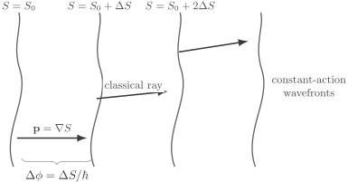
On a smooth branch, the local momentum $\mathbf p=\nabla S$ is normal to the constant-action fronts. An action increment $\Delta S$ between fronts produces the relative phase $\Delta\phi=\Delta S/\hbar$.

Phase velocity is not particle velocity

For a plane action

$$S(\mathbf x,t) = \mathbf p\mathbin{\cdot}\mathbf x - Et,$$

a constant-phase plane moves in the normal direction with phase velocity

$$v_{\mathrm{ph}} = \frac{E}{\lvert\mathbf p\rvert}.$$

For a nonrelativistic free particle, $E=p^2/(2m)$, so

$$v_{\mathrm{ph}} = \frac{\lvert p\rvert}{2m}.$$

The Hamiltonian ray and wave-packet group velocity are instead

$$v_{\mathrm{ray}} = v_{\mathrm g} = \frac{\partial E}{\partial p} = \frac{p}{m}.$$

Following a phase crest is therefore not the same as following a particle or packet center. Group Velocity and Phase Velocity owns the full wave-packet distinction.

Action as an Endpoint Generator

Let a classical trajectory branch $\gamma$ connect $(q_i,t_i)$ to $(q_f,t_f)$. Its on-shell action is

$$S_\gamma(q_f,t_f;q_i,t_i) = \int_{t_i}^{t_f} L(q_\gamma,\dot q_\gamma,t)\,dt.$$

Varying the endpoints while keeping the path on shell gives

$$\begin{aligned} dS_\gamma ={}& p_f\mathbin{\cdot}dq_f - H_f\,dt_f \\ &- p_i\mathbin{\cdot}dq_i + H_i\,dt_i. \end{aligned}$$

Hence

$$\begin{aligned} p_f&=\nabla_{q_f}S_\gamma, & p_i&=-\nabla_{q_i}S_\gamma, \\ \partial_{t_f}S_\gamma&=-H_f, & \partial_{t_i}S_\gamma&=H_i. \end{aligned}$$

These signs matter. The same function generates both endpoint momenta because the initial and final endpoints enter with opposite orientation.

Second derivatives of $S_\gamma$ measure how the endpoint map responds to perturbations. They later become the Van Vleck determinant in the semiclassical propagator.

Action along a trajectory

In phase-space form,

$$dS = p_j\,dq^j - H\,dt.$$

Dividing by $\hbar$ gives the local phase increment

$$d\phi = \frac{1}{\hbar} \left( p_j\,dq^j - H\,dt \right).$$

Spatial translation accumulates phase through momentum; time evolution accumulates phase through energy. This is the differential form behind the plane-wave expression $\mathbf p\cdot\mathbf x-Et$.

The Hamilton–Jacobi Equation

Hold the initial endpoint fixed and consider one smooth action branch $S(q,t)$. The endpoint dictionary inserted into the Hamiltonian gives

$$\frac{\partial S}{\partial t} + H\left( q, \nabla S, t \right) = 0.$$

For a scalar potential,

$$H(q,p,t) = \frac{p^2}{2m} + V(q,t),$$

so

$$\frac{\partial S}{\partial t} + \frac{(\nabla S)^2}{2m} + V = 0.$$

This nonlinear first-order equation propagates phase fronts along classical characteristics. Hamilton–Jacobi Theory develops its complete integrals, generating functions, and canonical transformations.

Time-independent systems

When $H$ has no explicit time dependence, a fixed-energy branch can be written

$$S(q,t;E) = W(q;E)-Et,$$

where $W$ is Hamilton’s characteristic function. It satisfies

$$H(q,\nabla W)=E.$$

In one dimension,

$$\frac{dW}{dx} = \pm \sqrt{2m\bigl(E-V(x)\bigr)} = \pm p(x).$$

Therefore

$$W_\pm(x;E) = \pm \int^x p(x';E)\,dx'.$$

These two momentum branches become the two traveling WKB phases.

When the Wavefunction Phase Is Classical

For an exact wavefunction on a nodal-free patch, write

$$\psi = A e^{iS/\hbar}, \qquad A\geq0.$$

Substitution into the scalar-potential Schrödinger equation gives the exact phase equation

$$\frac{\partial S}{\partial t} + \frac{(\nabla S)^2}{2m} + V + Q = 0,$$

with

$$Q = - \frac{\hbar^2}{2m} \frac{\nabla^2A}{A}.$$

The amplitude also obeys the continuity equation

$$\partial_t(A^2) + \nabla\mathbin{\cdot} \left( A^2 \frac{\nabla S}{m} \right) = 0.$$

Thus the phase of an arbitrary exact wavefunction is not automatically a classical principal function. It becomes one at leading order only when the amplitude-dependent term $Q$ is small on the scale of the other Hamilton–Jacobi terms.

If $A$ varies over length $L_A$ and $p=\lvert\nabla S\rvert$, then

$$\frac{\lvert Q\rvert} {p^2/(2m)} \sim \left( \frac{\hbar}{pL_A} \right)^2.$$

The detailed exact derivation, node caveats, and multi-branch warning belong to Hamilton–Jacobi Theory Preview.

Action Differences Produce Interference

Suppose two semiclassical alternatives contribute

$$\mathcal M \approx A_1e^{iS_1/\hbar} + A_2e^{iS_2/\hbar}.$$

Then

$$\begin{aligned} \lvert\mathcal M\rvert^2 ={}& \lvert A_1\rvert^2 + \lvert A_2\rvert^2 \\ &+ 2\operatorname{Re} \left[ A_1A_2^* e^{i(S_1-S_2)/\hbar} \right]. \end{aligned}$$

The action difference supplies the interference phase

$$\Delta\phi = \frac{S_1-S_2}{\hbar}.$$

A common additive constant in both actions cancels. A difference of order $\hbar$ can shift an interference pattern by order one, even when both actions are individually enormous.

Why stationary action matters

In an oscillatory integral or regulated path integral, nonstationary changes in action produce rapidly changing phases. Neighboring contributions tend to cancel. Around a stationary path,

$$\delta S[q_\gamma]=0,$$

so the phase changes only at second order under nearby fixed-endpoint variations. A coherent neighborhood survives and produces the leading saddle contribution.

Stationary action is not maximum probability. Real-time factors $e^{iS/\hbar}$ have unit modulus for real $S$. Stationary Phase owns the asymptotic theorem; Action and Phase owns the path-history interpretation.

Free-Particle Example

For a free particle in $d$ dimensions and elapsed time $T=t_f-t_i\gt0$, the classical path is straight and

$$S_{\mathrm{free}} = \frac{m\lvert q_f-q_i\rvert^2}{2T}.$$

The endpoint derivatives give

$$\nabla_{q_f}S_{\mathrm{free}} = \frac{m(q_f-q_i)}{T} = p_f,$$

and

$$\partial_{t_f}S_{\mathrm{free}} = - \frac{m\lvert q_f-q_i\rvert^2}{2T^2} = - \frac{p_f^2}{2m}.$$

The exact propagator is

$$\begin{aligned} K_{\mathrm{free}} ={}& \left( \frac{m}{2\pi i\hbar T} \right)^{d/2} \\ &\times \exp\left[ \frac{i}{\hbar} S_{\mathrm{free}} \right]. \end{aligned}$$

The action supplies the phase; the prefactor supplies normalization and spreading. Because the free action is quadratic, the stationary-phase calculation is exact after the Gaussian normalization is included.

From Local Action to WKB

For a time-independent one-dimensional problem, the characteristic functions

$$W_\pm(x) = \pm\int^x p(x')\,dx'$$

give the leading local branches

$$\psi_\pm(x) \propto \exp\left[ \frac{i}{\hbar}W_\pm(x) \right].$$

This phase-only expression is not yet a WKB solution. The transport equation adds the amplitude $p^{-1/2}$, and turning-point matching connects branches globally. WKB Approximation is the canonical derivation.

Forbidden regions as complex action

Where $V(x)\gt E$, the local momentum is imaginary:

$$\begin{aligned} p(x) &= \pm i\kappa(x), \\ \kappa(x) &= \sqrt{2m\bigl(V(x)-E\bigr)}. \end{aligned}$$

The action branch becomes complex,

$$W_\pm(x) = \pm i \int^x\kappa(x')\,dx',$$

and the phase factor becomes exponential:

$$e^{iW_\pm/\hbar} = \exp\left[ \mp \frac{1}{\hbar} \int^x\kappa(x')\,dx' \right].$$

This analytic continuation explains the WKB decay and growth branches. It does not describe an ordinary real classical particle traveling under the barrier.

From Endpoint Action to Propagators

When several classical trajectories connect the same endpoints, each branch contributes its own action phase:

$$K_{\mathrm{sc}} \sim \sum_\gamma \mathcal A_\gamma \exp\left[ \frac{i}{\hbar}S_\gamma - i\frac{\pi}{2}\nu_\gamma \right].$$

The prefactor $\mathcal A_\gamma$ contains stability and normalization. The integer $\nu_\gamma$ tracks the phase change when the projected classical branch passes through caustics. The Semiclassical Propagator and Maslov Index own those structures.

At a caustic, a coordinate-space action branch can become multivalued or its prefactor can diverge. The underlying classical flow need not be singular; its projection into the chosen coordinates is. A different representation or uniform approximation repairs the quantum formula.

Gauge-Covariant Action Phase

For a particle of charge $q$ in electromagnetic potentials $(\Phi,\mathbf A)$, the Hamiltonian is

$$H = \frac{1}{2m} \left( \mathbf p-q\mathbf A \right)^2 + q\Phi.$$

The Hamilton–Jacobi equation becomes

$$\partial_tS + \frac{1}{2m} \left( \nabla S-q\mathbf A \right)^2 + q\Phi = 0.$$

Here

$$\mathbf p_{\mathrm{can}} = \nabla S$$

is canonical momentum, while

$$\boldsymbol\pi = \nabla S-q\mathbf A = m\mathbf v$$

is kinetic momentum.

Under the gauge transformation

$$\begin{aligned} \mathbf A'&=\mathbf A+\nabla\chi, \\ \Phi'&=\Phi-\partial_t\chi, \\ S'&=S+q\chi, \end{aligned}$$

the combinations

$$\nabla S-q\mathbf A$$

and

$$\partial_tS+q\Phi$$

are invariant. The wavefunction transforms consistently as

$$\psi' = e^{iq\chi/\hbar}\psi.$$

Therefore $\nabla S$ alone is not a gauge-invariant mechanical momentum. Local Phase Transformations and Minimal Coupling own the full gauge-covariant formalism.

Closed-loop electromagnetic phases can remain observable even where local fields vanish along the path. Their canonical physical treatment is the Aharonov–Bohm Effect, not this semiclassical dictionary page.

Boundary Terms and Phase Conventions

Adding a total derivative to a Lagrangian,

$$L' = L + \frac{dF(q,t)}{dt},$$

does not change the interior Euler–Lagrange equations. It changes the action by endpoint terms:

$$S' = S + F(q_f,t_f) - F(q_i,t_i).$$

A fixed-endpoint propagator therefore transforms by endpoint phases,

$$K' = e^{iF_f/\hbar} K e^{-iF_i/\hbar}.$$

Predictions remain unchanged when endpoint states and operators are transformed consistently. A classically irrelevant total derivative can thus change the phase convention of a quantum amplitude without changing its physics.

Where the Dictionary Needs Repair

Nodes

At $A=0$, the polar decomposition $\psi=Ae^{iS/\hbar}$ is singular. Phase winding around nodes can still carry physical information, but no single smooth local $S$ crosses the node.

Superposed branches

If

$$\psi = \sum_\gamma A_\gamma e^{iS_\gamma/\hbar},$$

the phase of the total sum is generally not equal to any $S_\gamma/\hbar$. The branch actions remain the useful semiclassical data; the total phase can jump near destructive-interference zeros.

Caustics

Several rays can project to one configuration-space point. The action becomes multivalued by branch, and the isolated prefactor fails. Use branch sums, Maslov phases, and a uniform approximation.

Gauge fields

Canonical phase gradients depend on gauge. Mechanical conclusions must use gauge-covariant combinations and closed-loop holonomies.

Strong amplitude variation

If $\hbar/(pL_A)$ is not small, the amplitude-dependent quantum term is not negligible. The exact wavefunction phase then need not obey the classical Hamilton–Jacobi equation.

Nonclassical saddles

Tunneling and other exponentially small effects may require complex action branches or Euclidean saddles. The slogan “phase equals classical action” must then include the chosen analytic continuation and contour.

Verification Checklist

Before interpreting an action as a quantum phase, ask:

1. Which action is meant: a path functional, principal function, characteristic function, or local wavefunction phase?
2. Is $S$ a real classical branch, a complex continuation, or the exact polar phase of a wavefunction?
3. Which endpoints, boundary conditions, and gauge convention define it?
4. Is the phase used only locally, or can nodes, loops, and caustics obstruct a global branch?
5. Are multiple classical branches present and, if so, have their amplitudes been added coherently?
6. Is the transport prefactor included when an amplitude rather than only a phase is claimed?
7. Is the amplitude-dependent quantum correction small in a stated dimensionless ratio?
8. Does the observable depend on an absolute convention or on a gauge-invariant relative phase?

Common Mistakes

• Saying $S/\hbar$ is large without identifying the action scale and observable.
• Treating the phase of an arbitrary exact wavefunction as a classical action with no amplitude correction.
• Confusing the path action functional $S[q]$ with an on-shell endpoint function $S_\gamma(q_f,t_f;q_i,t_i)$.
• Forgetting the minus sign in $E=-\partial_tS$.
• Identifying phase velocity with particle or group velocity.
• Treating $\nabla S$ as kinetic momentum in an electromagnetic field.
• Adding probabilities rather than amplitudes for several action branches.
• Ignoring endpoint phases induced by boundary terms or gauge transformations.
• Continuing a single phase branch through nodes or caustics.
• Reading an imaginary under-barrier momentum as an ordinary real-time classical trajectory.
• Keeping $e^{iS/\hbar}$ while omitting the prefactor and still claiming a normalized semiclassical amplitude.

Exercises

1. Plane-wave dictionary

For

$$\psi(\mathbf x,t) = A \exp\left[ \frac{i}{\hbar} \left( \mathbf p\mathbin{\cdot}\mathbf x -Et \right) \right],$$

verify the local momentum, energy, wavevector, and angular-frequency relations.

Solution

The action function is

$$S(\mathbf x,t) = \mathbf p\mathbin{\cdot}\mathbf x-Et.$$

Therefore

$$\nabla S=\mathbf p, \qquad -\partial_tS=E.$$

Since $\phi=S/\hbar$,

$$\mathbf k = \nabla\phi = \frac{\mathbf p}{\hbar},$$

and

$$\omega = -\partial_t\phi = \frac{E}{\hbar}.$$

2. Endpoint derivatives of the free action

For

$$S_{\mathrm{free}}(x_f,T;x_i,0) = \frac{m(x_f-x_i)^2}{2T},$$

compute $\partial S/\partial x_f$, $\partial S/\partial x_i$, and $\partial S/\partial T$.

Solution

The spatial derivatives are

$$\frac{\partial S}{\partial x_f} = \frac{m(x_f-x_i)}{T} = p_f,$$

and

$$\frac{\partial S}{\partial x_i} = - \frac{m(x_f-x_i)}{T} = -p_i.$$

For the straight free path, $p_i=p_f=p$. The time derivative is

$$\frac{\partial S}{\partial T} = - \frac{m(x_f-x_i)^2}{2T^2} = - \frac{p^2}{2m} = -E.$$

3. Action resolution of an interferometer

Two paths have action difference $\Delta S$. What action change shifts their relative phase by one full fringe? What action change exchanges constructive and destructive interference?

Solution

The relative phase is

$$\Delta\phi = \frac{\Delta S}{\hbar}.$$

One full fringe requires $\Delta\phi=2\pi$, so

$$\Delta S=2\pi\hbar=h.$$

Changing constructive interference into destructive interference requires a phase shift of $\pi$, hence an action change

$$\delta(\Delta S) = \pi\hbar = \frac{h}{2}.$$

4. A total derivative

Let $L'=L+dF(q,t)/dt$. Derive the phase relating the two fixed-endpoint propagators.

Solution

The actions differ by

$$S'[q]-S[q] = F(q_f,t_f)-F(q_i,t_i).$$

Every path with the same endpoints receives the same factor. With

$$F_f=F(q_f,t_f), \qquad F_i=F(q_i,t_i),$$

the result is

$$K'_{fi} = \exp\left[ \frac{i}{\hbar}F_f \right] K_{fi} \exp\left[ - \frac{i}{\hbar}F_i \right].$$

This is an endpoint phase convention; consistent transformation of states leaves physical amplitudes unchanged.

5. Gauge-covariant momentum

Show that $\nabla S-q\mathbf A$ and $\partial_tS+q\Phi$ are invariant under

$$\begin{aligned} \mathbf A' &= \mathbf A+\nabla\chi, \\ \Phi' &= \Phi-\partial_t\chi, \\ S' &= S+q\chi. \end{aligned}$$

Solution

For the spatial combination,

$$\begin{aligned} \nabla S'-q\mathbf A' &= \nabla S+q\nabla\chi -q\mathbf A-q\nabla\chi \\ &= \nabla S-q\mathbf A. \end{aligned}$$

For the temporal combination,

$$\begin{aligned} \partial_tS'+q\Phi' &= \partial_tS+q\partial_t\chi +q\Phi-q\partial_t\chi \\ &= \partial_tS+q\Phi. \end{aligned}$$

The Hamilton–Jacobi equation written from these combinations is therefore gauge invariant.

6. Phase and group velocities

For a free nonrelativistic particle with $E(p)=p^2/(2m)$, compute the phase velocity $E/p$ and group velocity $dE/dp$. Why is the second the ray velocity?

Solution

The phase velocity is

$$v_{\mathrm{ph}} = \frac{E}{p} = \frac{p}{2m}.$$

The group velocity is

$$v_{\mathrm g} = \frac{dE}{dp} = \frac{p}{m}.$$

Hamilton’s equation gives

$$\dot x = \frac{\partial H}{\partial p} = \frac{p}{m},$$

so the group velocity equals the Hamiltonian characteristic or ray velocity. A constant phase crest moves at a different speed.

References

1. H. Goldstein, C. Poole, and J. Safko, Classical Mechanics, 3rd ed. (Addison-Wesley, 2002). Hamilton’s principal function, endpoint derivatives, and Hamilton–Jacobi theory.
2. V. I. Arnold, Mathematical Methods of Classical Mechanics, 2nd ed. (Springer, 1989). Geometric formulation of action functions and Hamiltonian characteristics.
3. L. D. Landau and E. M. Lifshitz, Quantum Mechanics: Non-Relativistic Theory, 3rd ed. (Butterworth-Heinemann, 1981). Action phases, WKB wave mechanics, and electromagnetic coupling.
4. M. V. Berry and K. E. Mount, “Semiclassical approximations in wave mechanics”, Reports on Progress in Physics 35, 315–397 (1972). Action branches, WKB, turning points, and multidimensional semiclassics.
5. L. S. Schulman, Techniques and Applications of Path Integration (Wiley, 1981). Endpoint actions, propagators, and semiclassical stationary phase.
6. M. C. Gutzwiller, Chaos in Classical and Quantum Mechanics (Springer, 1990). Principal functions, classical trajectories, stability, and propagator phases.
7. Y. Aharonov and D. Bohm, “Significance of electromagnetic potentials in the quantum theory”, Physical Review 115, 485–491 (1959). Canonical example of gauge-invariant relative phase from electromagnetic holonomy.