t–J Model

The t–J model is a low-energy theory of mobile, spinful carriers in a Hilbert space from which local double occupancy has been removed. In quantum materials it is used most often as a deliberately compressed description of a doped Mott or charge-transfer insulator: charge moves at a scale set by hopping, while occupied neighboring sites exchange spin at a lower scale.

A materials calculation rarely stops at the nearest-neighbor textbook form. A useful ledger is

$$\begin{aligned} H_{\mathrm{mat}} ={}& -\sum_{i<j,\sigma} t_{ij}\, \mathcal P_G \left( c_{i\sigma}^{\dagger}c_{j\sigma} +\mathrm{h.c.} \right) \mathcal P_G \\ &+ \sum_{i<j} J_{ij} \left( \mathbf S_i\cdot\mathbf S_j -\frac14 n_i n_j \right) +H_{\mathrm{3s}} +H_{\mathrm{ring}} +H_{\mathrm{other}} . \end{aligned}$$

Here $\mathcal P_G=\prod_i(1-n_{i\uparrow}n_{i\downarrow})$ projects onto empty or singly occupied effective sites. The terms $H_{\mathrm{3s}}$, $H_{\mathrm{ring}}$, and $H_{\mathrm{other}}$ stand for correlated three-site motion, cyclic exchange, longer-range interactions, phonon couplings, disorder, or other operators generated by the reduction. Writing them explicitly in the ledger is a reminder that “the t–J model” is a family of effective theories, not a universal two-parameter law.

Canonical Scope

The t–J Model Preview is the canonical home for the constrained local Hilbert space, projected-operator algebra, standard Hamiltonian conventions, exact limits, finite-size formulation, and generic diagnostics. The Hubbard Model owns the parent one-band model, while Effective Hamiltonians in Many-Body Systems owns the block-diagonalization machinery and the detailed second-order derivation.

This page owns a different question:

When does a projected t–J description faithfully represent a quantum material, what measurements can calibrate it, and which cuprate claims remain model-dependent?

The derivation below therefore keeps a scale and operator ledger rather than repeating the full canonical algebra.

Strong-Coupling Route from the Hubbard Model

Split the one-band Hubbard Hamiltonian into an interaction $H_U=U D$, where $D=\sum_i n_{i\uparrow}n_{i\downarrow}$ counts doublons, and hopping pieces $T_m$ that change $D$ by $m=0,\pm1$. Let $P$ project onto the no-doublon sector and $Q=1-P$. For $U$ larger than every retained hopping scale and every target excitation energy, a Schrieffer–Wolff transformation gives

$$\begin{aligned} H_{\mathrm{eff}} ={}& P T_0 P - \frac{1}{U} P T_{-1}T_{+1}P \\ &+ O\!\left( \frac{\lVert T\rVert^3}{U^2} \right). \end{aligned}$$

The two displayed terms have distinct physical roles.

• $P T_0P$ is real hopping within the low-energy sector. It survives at first order when an empty site is available.
• $-PT_{-1}T_{+1}P/U$ describes a virtual excursion through a doublon. On one bond it produces antiferromagnetic exchange with $J_{ij}=4\lvert t_{ij}\rvert^2/U$ in the simplest one-band convention.

At exactly one electron per site, projected hopping is blocked and the leading nonconstant dynamics is spin exchange. Upon hole doping, projected hopping immediately reappears at order $t$, while exchange remains of order $t^2/U$. This separation explains why a single doped carrier can strongly disturb an antiferromagnetic background even when $J/t$ is numerically modest.

Controlled does not mean complete

The displayed expansion is controlled when $\lVert T\rVert/U\ll1$, but truncating it to projected hopping plus pairwise exchange makes an additional approximation. A two-step path $i\to j\to k$ through a virtual doublon generates correlated three-site hopping at order $t_{ij}t_{jk}/U$, the same order as $J$. At fourth order, one obtains corrections to pairwise exchange and cyclic exchange around plaquettes. Longer-range parent hoppings produce $t'$, $t''$, and mixed exchange processes.

Consequently, these statements are different:

1. the no-doublon effective theory is organized in powers of $t/U$;
2. the nearest-neighbor two-parameter t–J Hamiltonian is accurate for a chosen observable;
3. a particular material is represented by a one-band Hubbard parent.

The first can be controlled while the second or third fails.

No Double Occupancy Is a Statement About the Effective Orbital

Each projected site has the three states

$$\lvert 0\rangle, \qquad \lvert\uparrow\rangle, \qquad \lvert\downarrow\rangle.$$

The excluded fourth state is a doublon of the chosen effective orbital. It need not correspond to two electrons on one atom, nor does the projection say that all microscopic charge fluctuations vanish. A Wannier orbital may contain metal and ligand weight, and a local low-energy state may be a composite of several atomic orbitals.

This distinction is essential in cuprates. In a hole representation, the insulating parent has approximately one $d_{x^2-y^2}$ hole on each Cu site, whereas an added hole has substantial O $2p$ character. If a ligand hole and the neighboring Cu spin bind into a low-energy singlet, that composite can be represented as an empty site of an effective one-band model. Projecting the resulting band does not project oxygen out of the real charge density.

Filling and the projected sum rule

For $N_s$ effective sites, define the hole concentration

$$x = 1-\frac{1}{N_s}\sum_i\langle n_i\rangle .$$

The projected space then contains $(1-x)N_s$ electrons on average and $xN_s$ empty sites. Summing over spin, the zero-temperature spectral weights of a strictly projected electron operator obey

$$\begin{array}{rcl} W_{\mathrm{rem}}&=&1-x,\\[3pt] W_{\mathrm{add}}&=&2x,\\[3pt] W_{\mathrm{low}}&=&1+x. \end{array}$$

Removal acts on occupied sites; addition may place either spin on an empty site. The missing weight belongs to high-energy sectors absent from the t–J Hilbert space. A strict t–J model therefore cannot by itself predict the upper Hubbard band or the transfer of weight between retained and discarded sectors. Those questions require the parent Hubbard or charge-transfer model together with a consistently transformed observable.

Antiferromagnetic Exchange in a Material

In the one-band nearest-neighbor limit, $J=4t^2/U$ is a clean benchmark. In a material, however, the measured exchange can contain several virtual paths:

• metal–ligand–metal superexchange;
• direct overlap and intersite Coulomb exchange;
• Hund coupling on metal or ligand orbitals;
• multiple active metal orbitals;
• spin–orbit-generated anisotropic exchange;
• cyclic processes around a plaquette.

For a three-band Cu–O model written in hole language, let $\Delta_{pd}=\epsilon_p-\epsilon_d$ be the ligand-to-metal charge-transfer energy, $t_{pd}$ the Cu–O hopping, and $U_d,U_p$ the local interactions. A commonly used fourth-order scale estimate is

$$J_{\mathrm{CuO}} \sim \frac{4t_{pd}^{\,4}}{\Delta_{pd}^{\,2}} \left( \frac{1}{U_d} + \frac{2}{2\Delta_{pd}+U_p} \right),$$

before geometry, oxygen–oxygen hopping, direct exchange, and covalency corrections are included. The formula shows why assigning a measured $J$ to $4t^2/U$ can conceal the actual virtual states.

Inelastic neutron scattering and resonant inelastic x-ray scattering constrain the spin dispersion. For La$_2$CuO$_4$, the zone-boundary dispersion is evidence that nearest-neighbor Heisenberg exchange alone is insufficient; cyclic exchange or an equivalent higher-order description is needed. A fit value called $J$ is therefore meaningful only together with the fitted Hamiltonian and momentum range. The broader taxonomy belongs in Exchange Interactions.

From a Cu–O Model to One Effective Band

The minimal orbital starting point for a CuO$_2$ plane retains one Cu $d_{x^2-y^2}$ orbital and the neighboring O $p_x,p_y$ orbitals. Schematically,

$$\begin{aligned} H_{pd} ={}& \epsilon_d\sum_i n_i^d + \epsilon_p\sum_{\ell}n_\ell^p + H_{t_{pd}} + H_{t_{pp}} \\ &+ U_d\sum_i n_{i\uparrow}^d n_{i\downarrow}^d + U_p\sum_\ell n_{\ell\uparrow}^p n_{\ell\downarrow}^p + H_{V_{pd}} . \end{aligned}$$

This is a charge-transfer problem, not merely a one-band Hubbard model with a large onsite penalty. A one-band reduction requires an additional local-state argument.

Zhang–Rice singlet

Let $L_{i\sigma}^{\dagger}$ create the symmetry-adapted ligand-hole combination surrounding Cu site $i$. The local spin singlet has the form

$$\lvert\mathrm{ZR};i\rangle = \frac{1}{\sqrt2} \left( d_{i\uparrow}^{\dagger}L_{i\downarrow}^{\dagger} - d_{i\downarrow}^{\dagger}L_{i\uparrow}^{\dagger} \right) \lvert\mathrm{vac}\rangle .$$

If this state is separated from local triplets, nonbonding oxygen states, and other orbital configurations, it can serve as the spinless “empty” state of a projected one-band description. Motion and overlap of these composite states then generate effective hoppings and interactions.

The reduction is useful, but its assumptions must be audited:

1. Local spectral isolation: the singlet must remain the relevant low-energy charged state over the doping, pressure, and temperature range of interest.
2. Orthogonalization: ligand combinations on neighboring Cu sites overlap, so constructing orthogonal effective orbitals changes hopping amplitudes and produces longer-range terms.
3. Orbital stability: apical oxygen, Cu $4s$, other Cu $3d$ orbitals, and lattice distortions must not enter the target window strongly.
4. Observable transformation: oxygen-resolved spectroscopy cannot be compared with a bare one-band operator without transforming that operator through the same reduction.
5. Energy-window discipline: a model that reproduces sub-eV spin and carrier dynamics need not reproduce several-eV charge-transfer excitations.

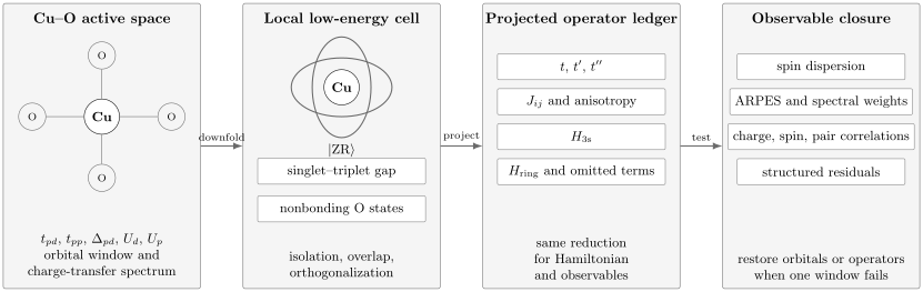
A material t–J description is a sequence of testable reductions. The active Cu–O window and local charged multiplets determine whether a one-band projected basis is justified; downfolding then generates a ledger containing $t_{ij}$, $J_{ij}$, three-site and ring terms. Validation must use transformed observables and should restore discarded orbitals or operators when residuals are structured.

Extended hopping is not cosmetic

The effective one-particle dispersion is often written

$$\begin{aligned} \varepsilon(\mathbf k) ={}& -2t(\cos k_x+\cos k_y) -4t'\cos k_x\cos k_y \\ &- 2t''(\cos2k_x+\cos2k_y) +\cdots . \end{aligned}$$

The ratios $t'/t$ and $t''/t$ change the location and curvature of low-energy states, magnetic frustration, stripe energetics, and pairing correlations in finite-cylinder calculations. Material trends in hopping range are tied to orbitals outside the nominal Cu $d_{x^2-y^2}$–O $p_\sigma$ manifold, including axial-orbital chemistry. Thus “same $J/t$” does not imply equivalent cuprates.

Doped Mott Insulators

At half filling, a projected carrier cannot hop to an occupied neighbor. A hole opens allowed first-order paths, but its motion permutes spins and accumulates fermionic signs. The resulting problem is not a dilute gas moving on a rigid antiferromagnet: charge motion reconstructs the spin correlations that in turn control charge coherence.

Several consequences follow without selecting a particular phase:

• the coherent bandwidth can be much smaller than the bare hopping scale;
• spectral weight is redistributed over energies of order both $t$ and $J$;
• antiferromagnetic correlations become incommensurate or short-ranged;
• holes may form polarons, stripes, bound pairs, or more homogeneous fluids depending on parameters and geometry;
• the signs and ranges of hopping matter, not only $J/t$;
• a finite cluster can favor an order that does not survive the two-dimensional and thermodynamic limits.

The t–J model is therefore a controlled descendant of a strong-coupling parent but generally a nonperturbative many-body problem in its own right.

Hole and electron doping are not mirror images

On a bipartite lattice, a particle–hole transformation can preserve the sign of nearest-neighbor hopping after a sublattice gauge choice. Same-sublattice hopping behaves differently:

$$t_{\mathrm{nn}}^{(h)}=t_{\mathrm{nn}}, \qquad t_{\mathrm{nnn}}^{(h)}=-t_{\mathrm{nnn}}.$$

This is one reason $t'$ is central to electron–hole asymmetry in one-band studies. Real cuprates add a deeper asymmetry: a doped electron tends toward a spinless Cu $d^{10}$ configuration, whereas a doped hole has strong ligand character and may form a Zhang–Rice-like state. A single projected band can encode some of this difference through parameters and operators, but it should not erase the distinct microscopic charge distributions.

What doping changes

Doping is not just a chemical-potential shift. It can change screening, effective interactions, orbital occupancies, lattice constants, disorder, and the energy separation to discarded states. A fixed-parameter t–J calculation answers a conditional question:

Given this projected Hamiltonian, how does its state evolve with carrier number?

It does not by itself prove that one Hamiltonian with fixed $t_{ij}$ and $J_{ij}$ describes an entire experimental doping series.

Cuprate Relevance

The t–J framework captures three robust pieces of cuprate phenomenology economically:

1. the parent compounds have strong short-range antiferromagnetic correlations;
2. doped carriers move in a Hilbert space with strongly suppressed local charge configurations;
3. spin, charge, and singlet-pair correlations compete on comparable low-energy scales.

It also provides a disciplined language for comparing projected variational states, tensor-network calculations, exact diagonalization, and effective gauge descriptions. The model has generated important hypotheses about resonating valence bonds, stripes, pseudogaps, and $d$-wave pairing.

What it does not establish by definition is equally important.

• It does not prove that every cuprate has a quantitatively valid one-band reduction.
• It does not prove that the nearest-neighbor $t$–$J$ Hamiltonian is the minimal adequate truncation.
• It does not identify the superconducting mechanism merely because the exchange term favors a bond singlet.
• It does not include oxygen-resolved charge-transfer excitations, the upper Hubbard band, phonons, long-range Coulomb forces, disorder, or structural layers unless these are added or encoded in transformed parameters.
• It does not make a finite-width cylinder identical to the two-dimensional thermodynamic system.

Why exchange suggests singlet pairing

Define the projected bond-singlet creator

$$B_{ij}^{\dagger} = \widetilde c_{i\uparrow}^{\dagger} \widetilde c_{j\downarrow}^{\dagger} - \widetilde c_{i\downarrow}^{\dagger} \widetilde c_{j\uparrow}^{\dagger}.$$

Within the projected space,

$$\mathbf S_i\cdot\mathbf S_j -\frac14n_i n_j = -\frac12 B_{ij}^{\dagger}B_{ij}.$$

The exchange interaction is therefore attractive in the occupied-bond singlet channel. A mean-field decoupling can produce a $d_{x^2-y^2}$ pattern because horizontal and vertical bond amplitudes may take opposite signs. But a local attractive channel is not yet superconductivity. A reliable bulk claim requires long-distance pair correlations or phase stiffness, careful comparison with charge order, control of truncation and boundary errors, and an extrapolation in both system length and width.

Recent tensor-network studies on finite cylinders find regimes with intertwined charge and pairing correlations and, for selected extended-model parameters, algebraically decaying $d$-wave correlations. These are important nonperturbative results. Their continuation to the isotropic two-dimensional thermodynamic limit, their parameter dependence, and their quantitative material mapping remain active research rather than settled theorem.

Model-to-Experiment Closure

No single observable validates a material t–J model. The strongest case uses one parameter set and one operator map across independent probes.

Question	Useful evidence	What must be reported
Is the spin sector right?	neutron or resonant x-ray spin dispersion, static susceptibility	fitted exchange network, anisotropy, ring terms, momentum and energy range
Is the carrier dispersion right?	angle-resolved photoemission, quantum oscillations where applicable	$t,t',t''$, self-energy convention, matrix elements, surface and doping conditions
Is projection adequate?	optical, x-ray absorption, inverse photoemission, charge-transfer spectroscopy	integrated weight window, transformed operators, omitted upper-band weight
Are competing orders reproduced?	x-ray and neutron scattering, scanning probes, thermodynamics	wave vector, correlation length, onset scale, disorder and finite-size sensitivity
Is superconductivity supported?	phase stiffness, penetration depth, Josephson response, pair-sensitive spectroscopy	symmetry, long-distance scaling, competing charge order, dimensional extrapolation

A practical validation loop is:

1. state the microscopic active space and energy window;
2. derive or fit every retained coupling in a declared basis;
3. transform the observables, not only the Hamiltonian;
4. compare several independent response functions;
5. vary plausible orbital windows and omitted operators;
6. interpret structured residuals as evidence for model revision.

Agreement with one dispersion after fitting several hoppings is calibration, not closure.

Common Mistakes

Treating projection as a large finite penalty

The t–J Hilbert space contains no doublon state. A Hubbard model with large but finite $U$ still contains doublons virtually and has high-energy spectral weight. The two descriptions agree only within a stated low-energy expansion and with consistently transformed operators.

Dropping three-site terms while claiming second-order accuracy

Exchange and three-site correlated hopping both scale as $t^2/U$. Keeping one and discarding the other may be a useful phenomenological truncation, but it is not the complete second-order Hubbard Hamiltonian away from half filling.

Using 4t²/U as a material identity

That expression belongs to a one-band, strong-coupling limit. Charge-transfer paths, orbital multiplets, direct exchange, and screening alter the material relation between hopping and spin exchange.

Calling every doped ligand hole an empty Cu site

The empty effective site may represent a composite local singlet with substantial oxygen density. Atom-resolved observables must retain that embedding.

Reading pairing from a short bond

The exchange term lowers a local singlet, so short-range pair correlations are expected. Superconductivity is a long-distance, phase-coherent statement and must be separated from a spin gap or local pair formation.

Ignoring the sign of longer-range hopping

Nearest-neighbor hopping alone has an enlarged particle–hole correspondence on a bipartite lattice. The sign of $t'$ breaks that simplification and can reorganize stripes, Fermi-surface geometry, and pairing correlations.

Using the model outside its energy window

A projected model cannot reproduce a charge-transfer excitation or upper Hubbard band that was integrated out. Adding a phenomenological broad feature does not restore the missing states or their sum rules.

Exercises

1. Order counting in the strong-coupling reduction

For a doped one-band Hubbard model, identify the leading orders in $t/U$ of projected nearest-neighbor hopping, exchange, three-site hopping, and plaquette ring exchange.

Solution

Projected hopping connects two states in the no-doublon sector directly, so its amplitude is order $t$.

Exchange and three-site hopping each require two hops with one virtual doublon denominator. Their scales are

$$J\sim\frac{t^2}{U}, \qquad t_{\mathrm{3s}}\sim\frac{t^2}{U}.$$

A four-site cyclic permutation requires four hops and three high-energy denominators in the simplest one-band process, so

$$K_{\mathrm{ring}} \sim \frac{t^4}{U^3}.$$

Numerical coefficients and additional denominators depend on the lattice and microscopic model. The central conclusion is that omitting three-site hopping is not justified by one extra power of $t/U$ relative to exchange.

2. Projected spectral-weight sum rule

A projected lattice has hole concentration $x$. Derive the total low-energy electron-removal and electron-addition weights per site, summed over spin.

Solution

An electron can be removed only from an occupied site. The average occupied fraction is $1-x$, hence

$$W_{\mathrm{rem}}=1-x.$$

An electron can be added only to an empty site. Each empty site accepts either spin, so

$$W_{\mathrm{add}}=2x.$$

Thus the projected low-energy total is

$$W_{\mathrm{low}} = W_{\mathrm{rem}}+W_{\mathrm{add}} = 1+x.$$

The result differs from the total two-spin-orbital weight $2$ of an unprojected one-band model. The missing $1-x$ resides in discarded high-energy addition states. At finite $U$, virtual mixing also transfers spectral weight dynamically, which is beyond the strict projected counting.

3. Exchange paths in a charge-transfer model

Using the schematic Cu–O estimate

$$J_{\mathrm{CuO}} \propto \frac{t_{pd}^{\,4}}{\Delta_{pd}^{\,2}} \left( \frac{1}{U_d} + \frac{2}{2\Delta_{pd}+U_p} \right),$$

determine how $J_{\mathrm{CuO}}$ changes under a small fractional increase $t_{pd}\to t_{pd}(1+\eta)$ with all other parameters fixed.

Solution

Because the displayed estimate is fourth order in $t_{pd}$,

$$\frac{J_{\mathrm{CuO}}(\eta)} {J_{\mathrm{CuO}}(0)} = (1+\eta)^4 = 1+4\eta+O(\eta^2).$$

The leading fractional change is therefore

$$\frac{\delta J_{\mathrm{CuO}}}{J_{\mathrm{CuO}}} \simeq 4\eta.$$

This strong sensitivity explains why bond geometry and covalency matter. In a real pressure or substitution series, however, $\Delta_{pd}$, screening, and orbital composition also change, so varying only $t_{pd}$ is a diagnostic rather than a complete material prediction.

4. Particle–hole transformation of t′

On a square bipartite lattice, take $c_{i\sigma}\mapsto\eta_i h_{i\sigma}^{\dagger}$ with $\eta_i=+1$ on sublattice A and $-1$ on sublattice B. Show why nearest-neighbor hopping preserves its sign while next-nearest-neighbor hopping changes sign in the hole Hamiltonian.

Solution

For $i\ne j$,

$$c_{i\sigma}^{\dagger}c_{j\sigma} \mapsto \eta_i\eta_j h_{i\sigma}h_{j\sigma}^{\dagger} = -\eta_i\eta_j h_{j\sigma}^{\dagger}h_{i\sigma}.$$

Comparing with the standard hopping form shows that the transformed amplitude is

$$t_{ij}^{(h)} = -\eta_i\eta_j t_{ij}.$$

Nearest neighbors lie on opposite sublattices, so $\eta_i\eta_j=-1$ and $t^{(h)}=t$. Next-nearest neighbors lie on the same sublattice, so $\eta_i\eta_j=+1$ and $t'^{(h)}=-t'$. Longer-range hopping therefore carries physically important electron–hole asymmetry.

5. Bond exchange and the singlet channel

Verify the identity

$$\mathbf S_i\cdot\mathbf S_j -\frac14 n_i n_j = -\frac12 B_{ij}^{\dagger}B_{ij}$$

on the empty, singly occupied, triplet, and singlet bond sectors.

Solution

If fewer than two electrons occupy the bond, both sides vanish: there is no pair for $B_{ij}$ to remove, and either $n_in_j=0$ or one spin operator is zero.

For two occupied sites, use

$$\mathbf S_i\cdot\mathbf S_j = \frac12 \left[ S_{\mathrm{tot}}(S_{\mathrm{tot}}+1) -\frac32 \right].$$

On a triplet, $S_{\mathrm{tot}}=1$, so the left side is $1/4-1/4=0$. The singlet annihilator also kills a triplet.

On a singlet, $S_{\mathrm{tot}}=0$, so the left side is $-3/4-1/4=-1$. With the unnormalized definition used above, $B_{ij}$ maps the normalized singlet to $\sqrt2\lvert0\rangle$, hence $B_{ij}^{\dagger}B_{ij}$ has eigenvalue $2$ and the right side is also $-1$.

6. Audit a one-band claim

Suppose a one-band t–J calculation reproduces the low-energy spin-wave velocity of a cuprate after fitting $J$, but misses the zone-boundary dispersion, oxygen-resolved x-ray weight, and doping dependence of the optical sum. Classify the evidence and propose the next model revision.

Solution

Matching the spin-wave velocity calibrates one low-energy combination of exchange parameters. It does not validate the full Hamiltonian.

The zone-boundary residual is structured in momentum and points toward longer-range or cyclic exchange. Missing oxygen-resolved weight is expected if the observable embedding or the oxygen orbitals themselves were discarded. Failure of the optical doping trend indicates that fixed projected-space sum rules or fixed parameters are inadequate over the stated window.

A disciplined revision would first add the exchange operators demanded by the spin dispersion and transform the x-ray and optical operators consistently. If the high-energy and doping-dependent residuals remain, the active space should be enlarged to a Cu–O charge-transfer model, with doping-dependent screening and orbital content tested rather than absorbed into an unconstrained fit.

Research Status

The strong-coupling reduction, projected Hilbert space, exchange scale, and need for generated terms are standard results. The usefulness of extended t–J models as low-energy organizers of cuprate spin and charge physics is also well established.

Active questions include the quantitative accuracy of one-band reductions across cuprate families and doping levels, the minimal set of longer-range and multiorbital terms, the two-dimensional thermodynamic phase diagram, and whether the model’s strongest pairing regimes explain the observed superconducting state without essential additional degrees of freedom. Numerical evidence should always be labeled by geometry, width, boundary conditions, parameter set, and extrapolation strategy.

Connections

• t–J Model Preview — projected operators, exact limits, finite-size formulation, and generic model diagnostics.
• Hubbard Model — the parent one-band Hamiltonian and its strong-coupling sectors.
• Effective Hamiltonians in Many-Body Systems — Schrieffer–Wolff construction, projectors, and generated operators.
• Hubbard Physics in Materials — active subspaces, screened interactions, double counting, and model validation.
• Mott Insulators — charge incompressibility, material mechanisms, and doping.
• Spectral Functions — addition and removal spectra and their sum rules.
• Equal-Time Correlations — finite-size diagnostics for spin, charge, and pair order.
• Charge and Spin Density Waves — material signatures, collective modes, and superconducting competition for stripes and other finite-wavevector orders.
• Variational Many-Body States — projected trial states and evidence standards.
• Exchange Interactions — superexchange, direct exchange, itinerant mechanisms, and anisotropy.

References

• K. A. Chao, J. Spałek, and A. M. Oleś, “Canonical perturbation expansion of the Hubbard model,” Physical Review B 18, 3453–3464 (1978).
• A. H. MacDonald, S. M. Girvin, and D. Yoshioka, “$t/U$ expansion for the Hubbard model,” Physical Review B 37, 9753–9756 (1988).
• V. J. Emery, “Theory of high-$T_c$ superconductivity in oxides,” Physical Review Letters 58, 2794–2797 (1987).
• F. C. Zhang and T. M. Rice, “Effective Hamiltonian for the superconducting Cu oxides,” Physical Review B 37, 3759–3761 (1988).
• J. H. Jefferson, H. Eskes, and L. F. Feiner, “Derivation of a single-band model for CuO$_2$ planes by a cell-perturbation method,” Physical Review B 45, 7959–7972 (1992).
• E. Dagotto, “Correlated electrons in high-temperature superconductors,” Reviews of Modern Physics 66, 763–840 (1994).
• P. A. Lee, N. Nagaosa, and X.-G. Wen, “Doping a Mott insulator: Physics of high-temperature superconductivity,” Reviews of Modern Physics 78, 17–85 (2006).
• B. Edegger, V. N. Muthukumar, and C. Gros, “Gutzwiller–RVB theory of high-temperature superconductivity: Results from renormalized mean-field theory and variational Monte Carlo calculations,” Advances in Physics 56, 927–1033 (2007).
• J.-Y. P. Delannoy, M. J. P. Gingras, P. C. W. Holdsworth, and A.-M. S. Tremblay, “Low-energy theory of the $t$–$t'$–$t''$–$U$ Hubbard model at half-filling,” Physical Review B 79, 235130 (2009).
• R. Coldea, S. M. Hayden, G. Aeppli, et al., “Spin waves and electronic interactions in La$_2$CuO$_4$,” Physical Review Letters 86, 5377–5380 (2001).
• E. Pavarini, I. Dasgupta, T. Saha-Dasgupta, O. Jepsen, and O. K. Andersen, “Band-structure trend in hole-doped cuprates and correlation with $T_{c,\max}$,” Physical Review Letters 87, 047003 (2001).
• H. Eskes, M. B. J. Meinders, and G. A. Sawatzky, “Anomalous transfer of spectral weight in doped strongly correlated systems,” Physical Review Letters 67, 1035–1038 (1991).
• R. S. Markiewicz, T. Das, and A. Bansil, “Failure of t–J models in describing doping evolution of spectral weight in x-ray scattering, optical, and photoemission spectra of cuprates,” Physical Review B 82, 224501 (2010).
• H.-C. Jiang, Z.-Y. Weng, and S. A. Kivelson, “Superconductivity in the doped t–J model: Results for four-leg cylinders,” Physical Review B 98, 140505(R) (2018).
• X. Lu, F. Chen, W. Zhu, D. N. Sheng, and S.-S. Gong, “Emergent superconductivity and competing charge orders in hole-doped square-lattice t–J model,” Physical Review Letters 132, 066002 (2024).
• N. P. Armitage, P. Fournier, and R. L. Greene, “Progress and perspectives on electron-doped cuprates,” Reviews of Modern Physics 82, 2421–2487 (2010).
• K. Sheshadri, D. Malterre, A. Fujimori, and A. Chainani, “Connecting the one-band and three-band Hubbard models of cuprates via spectroscopy and scattering experiments,” Physical Review B 107, 085125 (2023).
• M. Hirayama, Y. Yamaji, T. Misawa, and M. Imada, “Ab initio effective Hamiltonians for cuprate superconductors,” Physical Review B 98, 134501 (2018).

Summary

A material t–J model is a projected, energy-window-dependent description whose parameters and operators inherit a microscopic embedding. The one-band Hubbard expansion explains projected hopping, antiferromagnetic exchange, and generated three-site terms, but a cuprate reduction must also justify the Zhang–Rice-like local state and account for Cu–O charge-transfer physics. Longer-range hopping, ring exchange, observable transformations, and doping-dependent screening are often essential. The model is a powerful organizer of doped-Mott competition and singlet correlations; it is not, by its name alone, proof of a unique cuprate Hamiltonian or superconducting mechanism.