WKB Bound States in a Smooth Potential

This worked example estimates the bound-state spectrum of a smooth confining potential from a classical action integral, then tests the estimate against independent numerical diagonalization. The model is the pure quartic oscillator,

$$H = \frac{p^2}{2m} + \lambda x^4, \qquad \lambda\gt0.$$

It is a particularly clean WKB test. The well has two ordinary turning points at every positive energy, but unlike the harmonic oscillator its leading WKB spectrum is not accidentally exact. The action can still be evaluated analytically, so any discrepancy with the numerical spectrum measures the semiclassical approximation rather than quadrature error.

Bohr–Sommerfeld Quantization is the canonical home for the general quantization rule and its Maslov correction. Turning Points and Connection Formulas owns the Airy matching that produces that correction. This page owns the complete quartic-oscillator calculation, including its scaling, analytic action, numerical benchmark, and error interpretation.

Problem Statement

For

$$V(x)=\lambda x^4,$$

find the leading WKB estimate of every bound-state energy $E_n$. Then answer four questions:

1. What dimensional combination of $m$, $\lambda$, and $\hbar$ sets the energy scale?
2. How does the spectrum grow with $n$?
3. How accurate is leading WKB for the first several levels?
4. Does the sign of the observed error imply a rigorous bound?

The state label is

$$n=0,1,2,\ldots,$$

with even and odd parity alternating as usual for a symmetric one-dimensional well.

Why WKB Is the Right Approximation

The target is an entire spectrum rather than a weak-coupling correction around another solvable Hamiltonian. There is no independent small coupling in the pure quartic model: a rescaling removes $\lambda$, $m$, and $\hbar$ from the dimensionless eigenvalue problem.

WKB is nevertheless asymptotically controlled for highly excited states. Their de Broglie wavelength changes little over most of a classical orbit, and the two regions where the local approximation fails can be treated by simple-turning-point connection formulas. The resulting action rule becomes increasingly accurate as the number of oscillations between the turning points grows.

This method choice also fixes what must be checked. We need:

• two isolated simple turning points;
• a correctly normalized half-orbit action;
• the $1/2$ Maslov shift from the two turning points;
• an independent solution of the original Schrödinger equation;
• a convergence test for that numerical solution.

Turning Points and Classical Regions

At a trial energy $E\gt0$, the turning-point equation is

$$E=\lambda x^4.$$

Its two real solutions are

$$x_\pm(E) = \pm a(E), \qquad a(E) = \left( \frac{E}{\lambda} \right)^{1/4}.$$

The interval $-a\lt x\lt a$ is classically allowed. The two exterior regions are forbidden and contain the decaying tails of a normalizable bound state.

Both turning points are simple because

$$V'(x_\pm) = 4\lambda x_\pm^3 \ne0 \qquad \text{for }E\gt0.$$

Thus the local potential is linear to leading order at each endpoint, Airy matching applies, and each endpoint contributes a phase of $\pi/4$. The stationary point at $x=0$ is not a turning point for a positive-energy orbit: there $V(0)=0\lt E$ and the classical momentum is nonzero.

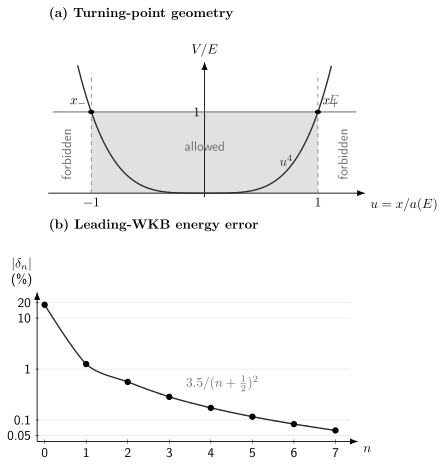
Top: in the scaled coordinate $u=x/a(E)$, the turning points are always $u=\pm1$ and the allowed region lies between them. Bottom: the absolute relative error of the leading WKB energies decreases rapidly with level number; the dashed line shows the observed $3.5/(n+1/2)^2$ percent asymptotic behavior.

Remove the Dimensional Parameters

Before integrating, identify the natural scales. Let

$$x=\ell q, \qquad \ell = \left( \frac{\hbar^2}{m\lambda} \right)^{1/6}.$$

The kinetic and potential coefficients then share the energy scale

$$E_* = \frac{\hbar^2}{m\ell^2} = \lambda\ell^4 = \left( \frac{\hbar^4\lambda}{m^2} \right)^{1/3}.$$

The stationary Schrödinger equation becomes

$$\left[ -\frac12\frac{d^2}{dq^2} + q^4 \right] \psi(q) = \epsilon\psi(q).$$

Here $\epsilon=E/E_*$ is dimensionless.

Every physical eigenvalue must therefore have the form

$$E_n=E_*\,\epsilon_n,$$

where $\epsilon_n$ is a pure number. This scaling is exact; only the estimate of $\epsilon_n$ will be semiclassical.

The scale already gives useful physics. A larger stiffness $\lambda$ raises all levels as $\lambda^{1/3}$, while a larger mass lowers them as $m^{-2/3}$. These exponents differ from harmonic-oscillator scaling because the quartic potential has no fixed frequency.

Evaluate the Action Integral

For a bound orbit, define the momentum in the allowed region by

$$p(x;E) = \sqrt{ 2m\left( E-\lambda x^4 \right) }.$$

The half-orbit action between the two turning points is

$$I(E) = \int_{-a}^{a}p(x;E)\,dx.$$

Symmetry gives

$$I(E) = 2\sqrt{2m} \int_0^a \sqrt{ E-\lambda x^4 } \,dx.$$

Set

$$x=au, \qquad a=\left(\frac{E}{\lambda}\right)^{1/4}.$$

Because $\lambda a^4=E$,

$$\begin{aligned} I(E) &= 2\sqrt{2m}\, a\sqrt{E} \int_0^1 \sqrt{1-u^4}\,du \\ &= 2C_4\sqrt{2m}\, \lambda^{-1/4}E^{3/4}, \end{aligned}$$

where the dimensionless integral is

$$C_4 \equiv \int_0^1 \sqrt{1-u^4}\,du.$$

To evaluate it, use $t=u^4$. Then

$$\begin{aligned} C_4 &= \frac14 \int_0^1 t^{-3/4}(1-t)^{1/2}\,dt \\ &= \frac14 B\left( \frac14,\frac32 \right). \end{aligned}$$

In gamma functions,

$$C_4 = \frac{ \sqrt{\pi}\, \Gamma(1/4) }{ 6\Gamma(3/4) } = 0.874019184764\ldots.$$

The beta function is not a decorative rewrite. It supplies the numerical coefficient that distinguishes the quartic spectrum from a scaling estimate alone. See Gamma and Beta Functions for the identities used here.

Impose the Quantization Condition

Two smooth turning points give the leading Bohr–Sommerfeld condition

$$I(E_n) = \pi\hbar \left( n+\frac12 \right).$$

Substituting the quartic action,

$$2C_4\sqrt{2m}\, \lambda^{-1/4}E_n^{3/4} = \pi\hbar \left( n+\frac12 \right).$$

Solving for the energy gives

$$E_n^{\mathrm{WKB}} = \left[ \frac{ \pi\hbar\lambda^{1/4} }{ 2C_4\sqrt{2m} } \left( n+\frac12 \right) \right]^{4/3}.$$

Equivalently,

$$\frac{ E_n^{\mathrm{WKB}} }{ E_* } = A_4 \left( n+\frac12 \right)^{4/3},$$

with

$$\begin{aligned} A_4 &= \left( \frac{\pi}{2\sqrt{2}\,C_4} \right)^{4/3} \\ &= 1.376507403471\ldots. \end{aligned}$$

This is the requested spectrum estimate. Its two most important structural features are the universal smooth-turning-point shift $n+1/2$ and the quartic growth law $E_n\propto n^{4/3}$.

Interpretation from the Classical Period

The closed-orbit action is twice the half-orbit action:

$$\begin{aligned} J(E) &= \oint p\,dx = 2I(E) \\ &= 4C_4\sqrt{2m}\, \lambda^{-1/4}E^{3/4}. \end{aligned}$$

For one-dimensional periodic motion,

$$\tau(E)=\frac{dJ}{dE}.$$

Therefore

$$\tau(E) = 3C_4\sqrt{2m}\, \lambda^{-1/4}E^{-1/4}.$$

The classical period decreases as the energy rises: a quartic oscillator becomes effectively stiffer at larger amplitude. Since adjacent semiclassical levels differ by $\Delta J=2\pi\hbar$,

$$\Delta E \simeq \frac{2\pi\hbar}{\tau(E)} \propto E^{1/4} \propto n^{1/3}.$$

Thus the widening quantum level spacing is the spectral image of the shortening classical period.

Independent Numerical Benchmark

To test WKB, solve the dimensionless Hamiltonian

$$\mathcal H = -\frac12\frac{d^2}{dq^2} + q^4$$

in a harmonic-oscillator basis of adjustable frequency $\Omega$. If

$$\mathcal H_\Omega = -\frac12\frac{d^2}{dq^2} + \frac12\Omega^2q^2,$$

then the matrix to diagonalize is assembled as

$$\mathcal H = \mathcal H_\Omega + q^4 - \frac12\Omega^2q^2.$$

The coordinate matrix follows from

$$q = \frac{ a+a^\dagger }{ \sqrt{2\Omega} },$$

so $q^2$ and $q^4$ can be formed by matrix multiplication before diagonalization. This solves the original quartic eigenvalue problem; it does not discretize the WKB condition.

For the values below, $\Omega=2$ and basis sizes $N=80$, $120$, and $180$ were compared. The largest change among the first eight eigenvalues between $N=120$ and $N=180$ was below $3\times10^{-12}$. Repeating the calculation with $\Omega=1$, $3$, and $4$ gave the displayed digits after increasing the basis size. The reference values are therefore numerically converged well beyond the precision needed to assess leading WKB.

Define the signed relative error by

$$\delta_n = \frac{ E_n^{\mathrm{WKB}}-E_n^{\mathrm{num}} }{ E_n^{\mathrm{num}} }.$$

All energies in the table are in units of $E_*$.

$n$	$E_n^{\mathrm{WKB}}/E_*$	$E_n^{\mathrm{num}}/E_*$	$100\delta_n$
0	0.546267325	0.667986259	$-18.2218\%$
1	2.363561445	2.393644016	$-1.25677\%$
2	4.670519932	4.696795387	$-0.55943\%$
3	7.314802602	7.335729995	$-0.28528\%$
4	10.226536434	10.244308455	$-0.17348\%$
5	13.363764206	13.379336553	$-0.11639\%$
6	16.697945033	16.711889633	$-0.08344\%$
7	20.208166094	20.220849464	$-0.06272\%$

The ground state is not semiclassical: there is too little phase accumulation between its turning points, and the leading estimate misses the energy by about $18\%$. The first excited state is already within about $1.3\%$, and levels with $n\ge2$ are within $0.6\%$ for this model.

For the displayed excited levels, the error is well described by

$$\left|\delta_n\right| \simeq \frac{ 0.035 }{ \left( n+\frac12 \right)^2 }.$$

This $n^{-2}$ behavior is consistent with the first omitted higher-order WKB correction after the leading action rule. It is an empirical asymptotic check for this model, not a universal error constant for arbitrary potentials.

What the Error Does and Does Not Prove

Every leading-WKB value in the table lies below the corresponding numerical value. That pattern is useful evidence about this model, but it does not turn WKB into a variational principle.

Rayleigh–Ritz upper bounds follow from evaluating the exact Hamiltonian in normalized trial states. WKB energies instead follow from truncating an asymptotic expansion and imposing approximate matching conditions. No general ordering theorem requires the neglected terms to have one sign. A different potential, level, boundary singularity, or WKB correction can reverse the sign of the error.

The defensible statement is therefore:

For the first eight pure-quartic levels, the leading smooth-turning-point WKB estimate underestimates the converged numerical energy, and its relative error decreases approximately as $(n+1/2)^{-2}$ beyond the lowest levels.

It would be an overclaim to call the formula a rigorous lower bound.

General Power-Law Check

The same calculation reveals why the exponent $4/3$ is natural. Consider

$$V(x) = \lambda|x|^\nu, \qquad \nu\gt0.$$

The turning point is $a=(E/\lambda)^{1/\nu}$, and

$$C_\nu \equiv \int_0^1 \sqrt{1-u^\nu}\,du = \frac1\nu B\left( \frac1\nu,\frac32 \right).$$

The half-orbit action is

$$I_\nu(E) = 2C_\nu\sqrt{2m}\, \lambda^{-1/\nu} E^{1/2+1/\nu}.$$

Leading WKB therefore gives

$$E_n^{\mathrm{WKB}} = \left[ \frac{ \pi\hbar\lambda^{1/\nu} }{ 2C_\nu\sqrt{2m} } \left( n+\frac12 \right) \right]^{2\nu/(\nu+2)}.$$

For $\nu=4$, this reduces to the quartic result. For $\nu=2$ and $\lambda=m\omega^2/2$, the integral has $C_2=\pi/4$ and the formula reduces to

$$E_n = \hbar\omega \left( n+\frac12 \right),$$

the exact harmonic-oscillator spectrum. This exactness is special: it should validate the normalization and turning-point phase, not be taken as typical leading-WKB accuracy.

Validity Audit

Turning-point structure

At every physical quartic eigenvalue, $x_\pm$ are isolated simple zeros of $E-V(x)$. Ordinary Airy connection formulas apply. The coalesced root at $E=0$ is irrelevant to the positive discrete spectrum.

Local WKB condition

Away from the endpoint layers, a useful diagnostic is

$$\eta(x) \equiv \hbar \frac{ \left|p'(x)\right| }{ p(x)^2 } \ll1.$$

This condition necessarily fails as $x\to x_\pm$, where $p\to0$. The calculation remains meaningful because Airy matching replaces WKB inside those narrow layers. Increasing $n$ enlarges the action in units of $\hbar$ and improves the overlap between the interior WKB region and the turning-point asymptotics.

Low-state limitation

The formal quantization rule produces a number for $n=0$, but producing a number is not the same as controlling its error. The numerical benchmark shows that the ground state lies outside the quantitatively accurate regime of leading WKB.

Numerical independence

The benchmark uses a basis representation of the differential Hamiltonian, not numerical integration of the action formula. Basis-size and frequency variation test the numerical truncation separately from the semiclassical error.

Boundary limitation

The $n+1/2$ shift belongs to two smooth turning points. It cannot be transferred unchanged to hard walls, singular endpoints, or higher-order turning points. Those systems require their own boundary phase analysis.

Common Mistakes

• Using $\oint p\,dx$ in a formula written for $\int_{x_-}^{x_+}p\,dx$, thereby introducing a factor-of-two error.
• Dropping the $1/2$ shift and reverting to the pre-WKB integer action rule.
• Counting $x=0$ as a turning point because $V'(0)=0$; a turning point requires $V(x)=E$.
• Treating the dimensional scaling $E_*\propto\lambda^{1/3}m^{-2/3}$ as though it fixed the numerical coefficient.
• Applying the leading formula to the ground state without an independent error estimate.
• Calling converged numerical eigenvalues “exact” without stating the truncation and convergence checks.
• Inferring a rigorous lower bound from the negative errors in one table.
• Comparing WKB and numerics in inconsistent Hamiltonian conventions, especially after rescaling the kinetic term.

Exercises

1. Recover the natural scales

Starting from $\ell=(\hbar^2/m\lambda)^{1/6}$, verify that the kinetic coefficient $\hbar^2/(m\ell^2)$ and the quartic coefficient $\lambda\ell^4$ are equal. Show that both equal $E_*=(\hbar^4\lambda/m^2)^{1/3}$.

Solution

The kinetic coefficient is

$$\begin{aligned} \frac{\hbar^2}{m\ell^2} &= \frac{\hbar^2}{m} \left( \frac{m\lambda}{\hbar^2} \right)^{1/3} \\ &= \hbar^{4/3} \lambda^{1/3} m^{-2/3}. \end{aligned}$$

The potential coefficient is

$$\begin{aligned} \lambda\ell^4 &= \lambda \left( \frac{\hbar^2}{m\lambda} \right)^{2/3} \\ &= \hbar^{4/3} \lambda^{1/3} m^{-2/3}. \end{aligned}$$

Thus both equal

$$\left( \frac{\hbar^4\lambda}{m^2} \right)^{1/3} = E_*.$$

2. Derive the period from the action

Differentiate the closed action

$$J(E) = 4C_4\sqrt{2m}\, \lambda^{-1/4}E^{3/4}$$

and verify the period quoted above. Use $\Delta J=2\pi\hbar$ to derive the large-$n$ spacing law.

Solution

Differentiation gives

$$\tau(E) = \frac{dJ}{dE} = 3C_4\sqrt{2m}\, \lambda^{-1/4}E^{-1/4}.$$

For adjacent semiclassical levels,

$$\Delta J \simeq \frac{dJ}{dE}\Delta E = \tau(E)\Delta E = 2\pi\hbar.$$

Therefore

$$\Delta E \simeq \frac{2\pi\hbar}{\tau(E)} \propto E^{1/4}.$$

Since $E_n\propto n^{4/3}$ at large $n$,

$$\Delta E_n\propto n^{1/3}.$$

3. Check the harmonic limit of the power-law formula

Set $\nu=2$ and $\lambda=m\omega^2/2$ in the general power-law result. Evaluate $C_2$ directly and recover the exact harmonic-oscillator energies.

Solution

The integral is the area of a quarter unit disk:

$$C_2 = \int_0^1 \sqrt{1-u^2}\,du = \frac{\pi}{4}.$$

The power-law formula has exponent

$$\frac{2\nu}{\nu+2}=1.$$

Its coefficient becomes

$$\begin{aligned} \frac{ \pi\hbar\lambda^{1/2} }{ 2C_2\sqrt{2m} } &= \frac{ \pi\hbar\sqrt{m\omega^2/2} }{ (\pi/2)\sqrt{2m} } \\ &= \hbar\omega. \end{aligned}$$

Hence

$$E_n = \hbar\omega \left( n+\frac12 \right).$$

4. Estimate how many levels are semiclassically accurate

Using

$$\left|\delta_n\right| \simeq \frac{0.035}{(n+1/2)^2},$$

estimate the first $n$ for which the relative error is below $1\%$. Compare with the numerical table.

Solution

Demand

$$\frac{0.035}{(n+1/2)^2} \lt 0.01.$$

Then

$$n+\frac12 \gt \sqrt{3.5} \approx 1.87,$$

so the asymptotic estimate suggests $n\ge2$. The table gives a $0.559\%$ error at $n=2$, in agreement with that prediction.

The formula predicts about $1.56\%$ at $n=1$, while the observed error is $1.26\%$. This is reasonably close, but it also shows why a fitted asymptotic law should not be treated as an exact finite-$n$ bound.

5. Is leading WKB a lower-bound method?

The table has $E_n^{\mathrm{WKB}}\lt E_n^{\mathrm{num}}$ for every displayed level. Does this prove that leading WKB gives a lower bound for the pure quartic spectrum? Explain what additional structure would be needed for a rigorous variational claim.

Solution

No. A finite collection of negative errors establishes a numerical pattern for those levels, not an ordering theorem for the full spectrum. Leading WKB is obtained by truncating an asymptotic expansion and applying approximate connection formulas. Neither operation supplies a fixed sign for the omitted terms.

A variational upper-bound claim would require normalized trial states and the Rayleigh–Ritz principle. A rigorous lower bound would require a separate comparison theorem, operator inequality, or certified enclosure method. The WKB calculation supplies none of these by itself.

Cross-Links

• WKB Approximation develops the local asymptotic expansion and its validity criteria.
• Turning Points and Connection Formulas derives the Airy matching and $\pi/4$ phase at each endpoint.
• Bohr–Sommerfeld Quantization owns the general bound-state action rule.
• WKB Versus Exact Spectrum Notebook develops a reproducible coupling sweep for a quadratic-plus-quartic well.
• Anharmonic Oscillator by Variational Methods studies a different approximation to the same pure-quartic scaling regime and explains its upper-bound status.
• Matrix Diagonalization covers the numerical eigenvalue machinery used for the benchmark.

References

1. L. D. Landau and E. M. Lifshitz, Quantum Mechanics: Non-Relativistic Theory, 3rd ed., §§46–50, Pergamon Press (1977).
2. C. M. Bender and S. A. Orszag, Advanced Mathematical Methods for Scientists and Engineers I, Chapter 10, Springer (1999).
3. J. L. Dunham, “The Wentzel–Brillouin–Kramers Method of Solving the Wave Equation,” Physical Review 41, 713–720 (1932), doi:10.1103/PhysRev.41.713.
4. M. V. Berry and K. E. Mount, “Semiclassical approximations in wave mechanics,” Reports on Progress in Physics 35, 315–397 (1972), doi:10.1088/0034-4885/35/1/306.
5. N. Fröman and P. O. Fröman, JWKB Approximation: Contributions to the Theory, North-Holland (1965).