Rectangular Barrier Tunneling

Rectangular barrier tunneling is the canonical exact model of quantum penetration through a classically forbidden region. A particle with energy below the barrier height has an evanescent wave inside the barrier, yet a nonzero transmitted wave can emerge on the other side because the barrier has finite width.

Use

$$V(x)= \begin{cases} 0, & x\lt 0,\\ V_0, & 0\lt x\lt a,\\ 0, & x\gt a. \end{cases}$$

The tunneling regime is

$$0\lt E\lt V_0.$$

This page is the canonical calculation for that sub-barrier regime. The companion Finite Potential Barrier page treats the same geometry across threshold, including above-barrier reflection and transmission resonances.

The value of $V$ at the two isolated interfaces is irrelevant. A constant particle mass and no delta-function interface terms are assumed, so both $\psi$ and $\psi'$ are continuous at $x=0$ and $x=a$. A common factor $e^{-iEt/\hbar}$ is suppressed.

Region Solutions

Outside the barrier, define

$$k=\frac{\sqrt{2mE}}{\hbar}.$$

Inside the barrier, define the decay constant

$$\kappa=\frac{\sqrt{2m(V_0-E)}}{\hbar}.$$

For a wave incident from the left, write

$$\psi_I(x)=e^{ikx}+r e^{-ikx}, \qquad x\lt 0,$$

inside the barrier,

$$\psi_{II}(x)=A e^{\kappa x}+B e^{-\kappa x}, \qquad 0\lt x\lt a,$$

and to the right of the barrier,

$$\psi_{III}(x)=t e^{ikx}, \qquad x\gt a.$$

The coefficients are determined by continuity of $\psi$ and $\psi'$ at $x=0$ and $x=a$.

The ansatz specifies a wave incident only from the left. There is no $e^{-ikx}$ term in region III because no wave is incident from $+\infty$.

Both exponentials are required in the finite barrier. Dropping $Ae^{\kappa x}$ merely because it grows with $x$ would be appropriate only if the forbidden region extended to $+\infty$. On the finite interval $0\lt x\lt a$, neither term diverges asymptotically, and the second interface generally excites both.

The four matching equations are

$$\begin{aligned} 1+r&=A+B,\\ ik(1-r)&=\kappa(A-B),\\ Ae^{\kappa a}+Be^{-\kappa a} &=t e^{ika},\\ \kappa\left(Ae^{\kappa a}-Be^{-\kappa a}\right) &=ik t e^{ika}. \end{aligned}$$

They determine $r$, $A$, $B$, and $t$ for unit incident amplitude.

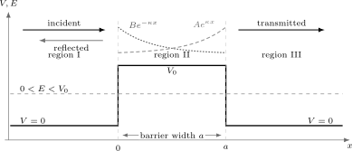
The tunneling ansatz for $0\lt E\lt V_0$. Region II requires both $Ae^{\kappa x}$ and $Be^{-\kappa x}$ because it is finite and matched at two interfaces. Each component alone has zero current; their matched coherent sum carries the constant current that emerges as the transmitted wave in region III. Curves and arrows are schematic.

Exact Transmission Amplitude

Inside the barrier, the endpoint data are related by

$$\begin{pmatrix} \psi(a)\\ \psi'(a) \end{pmatrix} = \begin{pmatrix} \cosh(\kappa a) & \sinh(\kappa a)/\kappa\\ \kappa\sinh(\kappa a) & \cosh(\kappa a) \end{pmatrix} \begin{pmatrix} \psi(0)\\ \psi'(0) \end{pmatrix}.$$

Substituting the incident/reflected data at $0$ and the outgoing data at $a$, then eliminating $r$, gives

$$t = \frac{e^{-ika}} {\displaystyle \cosh(\kappa a) +i\frac{\kappa^2-k^2}{2k\kappa} \sinh(\kappa a)}.$$

With the denominator denoted by $D$, the reflection amplitude is

$$r = -i\frac{k^2+\kappa^2}{2k\kappa} \frac{\sinh(\kappa a)}{D}.$$

The phase factor $e^{-ika}$ in $t$ depends on the convention for where the transmitted coefficient is referenced; it does not affect $T$. The phase of $t$ does affect wave-packet shifts and time-delay analyses, which require more care than the transmission probability alone.

Transmission Coefficient

For equal potentials on the left and right, the incident and transmitted wave numbers are the same. The transmission coefficient is therefore

$$T=\lvert t\rvert^2.$$

Solving the matching equations gives

$$T =\left[ 1+\frac{V_0^2\sinh^2(\kappa a)} {4E(V_0-E)} \right]^{-1}.$$

This follows from

$$\lvert D\rvert^2 =1+ \frac{(k^2+\kappa^2)^2}{4k^2\kappa^2} \sinh^2(\kappa a),$$

together with

$$k^2+\kappa^2=\frac{2mV_0}{\hbar^2}.$$

The reflection coefficient is

$$R=1-T$$

for this conservative one-dimensional problem.

Equivalently,

$$R = \frac{V_0^2\sinh^2(\kappa a)} {4E(V_0-E)+V_0^2\sinh^2(\kappa a)}.$$

Defining an energy fraction and barrier strength,

$$\epsilon=\frac{E}{V_0}, \qquad \alpha=a\frac{\sqrt{2mV_0}}{\hbar},$$

puts the result in the dimensionless form

T(\epsilon,\alpha) =left[ 1+ \frac{ \sinh^2\left(\alpha\sqrt{1-\epsilon}\right) }{4\epsilon(1-\epsilon)} \right]^{-1}, \qquad 0\lt\epsilon\lt1.

Thus every rectangular tunneling curve collapses to a two-parameter dimensionless family: the incident energy fraction and one strength-width parameter.

Worked Example: Mid-Barrier Energy

At $E=V_0/2$, the outside wave number and barrier decay constant are equal:

$$k=\kappa =\frac{\sqrt{mV_0}}{\hbar}.$$

The imaginary term in the exact denominator of $t$ vanishes, leaving

$$t=e^{-ika}\operatorname{sech}(\kappa a), \qquad T=\operatorname{sech}^2(\kappa a).$$

For $\kappa a=1$, $T\approx0.420$. For $\kappa a=3$, $T\approx9.87\times10^{-3}$, already close to the opaque approximation $4e^{-6}\approx9.92\times10^{-3}$. This example cleanly separates the exact hyperbolic dependence from its large-width exponential limit.

Opaque-Barrier Approximation

If the barrier is thick or high enough that

$$\kappa a\gg 1,$$

then

$$\sinh^2(\kappa a)\approx \frac14 e^{2\kappa a}.$$

The transmission coefficient is approximately

$$T \approx \frac{16E(V_0-E)}{V_0^2}e^{-2\kappa a}.$$

The most important dependence is exponential:

$$T\propto e^{-2\kappa a}.$$

Small changes in barrier width, particle mass, barrier height, or energy can cause large changes in tunneling probability.

More precisely,

$$\ln T \approx \ln\left[ \frac{16E(V_0-E)}{V_0^2} \right] -2\kappa a,$$

so at fixed $E$ and $V_0$,

$$\frac{\partial\ln T}{\partial a} \approx-2\kappa.$$

The exponent is exactly the rectangular-barrier WKB action,

$$2\kappa a =\frac{2}{\hbar} \int_0^a \sqrt{2m(V_0-E)}\,dx.$$

WKB reproduces the dominant exponential for a general smooth forbidden region, while the exact rectangular result supplies the interface-dependent prefactor. The opaque approximation must not be used near $E=V_0$ unless $\kappa a$ is still large.

Limiting Cases

• Zero width: As $a\to0$ at fixed $V_0$, $\sinh(\kappa a)\to0$ and $T\to1$.
• Zero incident energy: As $E\to0^+$ at fixed barrier, the exact denominator diverges and $T\to0$.
• Barrier top: As $E\to V_0^-$, both $\kappa$ and $\sinh(\kappa a)$ vanish, but their ratio with $V_0-E$ has a finite limit. With $k_0=\sqrt{2mV_0}/\hbar$,

$$T(E=V_0) =\left[ 1+\frac{k_0^2a^2}{4} \right]^{-1}.$$

This is nonzero because the zero-kinetic-energy region has finite width. It contrasts with the semi-infinite step, whose threshold transmission current is zero.

• Delta-barrier limit: Let $a\to0$ and $V_0\to\infty$ while $g=V_0a$ remains fixed. Then

T \longrightarrow \left[ 1+left( \frac{mg}{\hbar^2k} \right)^2 \right]^{-1},

the transmission probability for a repulsive delta barrier $g\delta(x)$.

For every nonzero rectangular barrier in the strict sub-barrier regime, $T\lt1$. Perfect resonant transmission belongs to the above-barrier regime, where the interior solution is oscillatory; that case is treated on Finite Potential Barrier.

Numerically Stable Evaluation

Directly evaluating $\sinh^2(\kappa a)$ can overflow for an opaque barrier even though the physically relevant answer is simply very small. A stable implementation should evaluate

$$\ln T =-\ln\left[ 1+C\sinh^2 s \right], \qquad C=\frac{V_0^2}{4E(V_0-E)}, \quad s=\kappa a,$$

using logarithmic functions such as a stable $\log(1+x)$ routine. For large $s$, use

$$\ln\sinh s =s-\ln2+\ln(1-e^{-2s})$$

rather than forming $e^s$ directly. In multilayer problems, multiplying ordinary transfer matrices can become ill-conditioned for the same reason; scattering-matrix or stabilized log-derivative methods are preferable.

Numerical checks should include $0\le T\le1$, $R+T=1$, agreement with the barrier-top limit, and convergence to the opaque asymptotic slope $d(\ln T)/da\to-2\kappa$.

Why Tunneling Is Not Step Penetration

For a semi-infinite step with $E\lt V_0$, the wavefunction decays into the forbidden region but carries no transmitted flux to infinity. For a finite barrier, there is a second boundary at $x=a$. The evanescent solution inside the barrier can match onto a propagating wave in region III.

The barrier interior is classically forbidden, but the wavefunction need not vanish there. The transmitted wave is not produced by the particle climbing over the barrier; it is a consequence of solving the wave equation with matching conditions across a finite forbidden region.

Energy is conserved throughout this time-independent problem. The phrase “classically forbidden” means that a classical point particle with total energy $E$ has no real local momentum in region II; it does not mean the quantum state temporarily violates energy conservation.

The stationary transmission coefficient also does not assign a unique trajectory or traversal time beneath the barrier. Several operational time concepts exist and need not coincide. Those questions require wave packets and measurement protocols beyond the scope of this probability calculation.

Probability Current

In regions I and III, the waves are propagating. The incident current is

$$j_{\text{inc}}=\frac{\hbar k}{m}.$$

The transmitted current is

$$j_{\text{trans}}=\frac{\hbar k}{m}\lvert t\rvert^2.$$

Thus, for equal potentials on the two sides,

$$T=\frac{j_{\text{trans}}}{j_{\text{inc}}}=\lvert t\rvert^2.$$

If the potentials differ on the two sides, a velocity factor must be included. Current ratios are the physical definitions.

There is an important interior subtlety. Each single exponential $Ae^{\kappa x}$ or $Be^{-\kappa x}$ carries zero current by itself, but their coherent superposition can carry current:

$$\begin{aligned} j_{II} &=\frac{\hbar}{m} \operatorname{Im}(\psi_{II}^*\psi_{II}')\\ &=\frac{2\hbar\kappa}{m} \operatorname{Im}(AB^*). \end{aligned}$$

Matching fixes a relative phase between $A$ and $B$ such that

$$j_{II} =j_{\mathrm{inc}}+j_{\mathrm{ref}} =j_{\mathrm{trans}},$$

where $j_{\mathrm{ref}}\lt0$. Tunneling current is therefore not carried by one decaying component moving classically through the barrier; it is a property of the full stationary solution across both interfaces.

Wave-Packet Transmission

For an incoming right-moving packet expanded in energy-normalized scattering states,

$$\int_0^\infty\lvert c(E)\rvert^2\,dE=1,$$

the late-time transmitted probability is

$$P_{\mathrm{trans}} =\int_0^\infty \lvert c(E)\rvert^2T(E)\,dE.$$

Only a spectrally narrow packet justifies $P_{\mathrm{trans}}\approx T(E_0)$. Because $T(E)$ grows rapidly with energy in the tunneling regime, the barrier preferentially transmits the high-energy side of a packet and can reshape it. If the initial energy distribution extends above $V_0$, that contribution is above-barrier transmission rather than tunneling.

Peak shifts in the transmitted packet do not by themselves define a traversal speed. Filtering and reshaping must be separated from causal signal propagation before drawing timing conclusions.

Physical Applications As First Encounters

Rectangular barriers are idealizations, but the exponential dependence they reveal is robust. Tunneling ideas appear in:

• alpha decay, where a nuclear particle tunnels through an effective Coulomb barrier;
• scanning tunneling microscopy, where current depends sensitively on tip-sample separation;
• Josephson junctions, where superconducting phase coherence changes the tunneling problem;
• tunnel diodes and semiconductor heterostructures;
• molecular inversion and double-well splitting.

These applications have richer canonical homes elsewhere. The rectangular barrier supplies the first exact one-dimensional calculation.

Only the qualitative mechanism and exponential sensitivity transfer directly. Alpha decay involves a radial Coulomb and centrifugal barrier, scanning tunneling currents also depend on electronic densities of states and matrix elements, and Josephson transport is coherent many-body pair tunneling. Quantitative work must use the appropriate Hamiltonian rather than substituting parameters into the rectangular prefactor.

Common Mistakes

• Setting the wavefunction to zero inside the barrier.
• Treating the barrier as semi-infinite and concluding $T=0$.
• Dropping the growing exponential inside a barrier of finite width.
• Concluding that the interior current vanishes because each exponential separately has zero current.
• Forgetting that the exponential is $e^{-2\kappa a}$ in probability, not $e^{-\kappa a}$.
• Using $T=\lvert t\rvert^2$ without checking whether the left and right wave numbers are equal.
• Using the opaque-barrier approximation when $\kappa a$ is not large, especially near the barrier top.
• Expecting perfect resonant transmission in the strict sub-barrier regime of one positive rectangular barrier.
• Interpreting tunneling as a temporary violation of energy conservation.
• Assigning a unique under-barrier trajectory or time from the stationary coefficient alone.
• Applying $T(E_0)$ to a broad packet instead of averaging over its energy distribution.
• Overflowing $\sinh(\kappa a)$ numerically instead of evaluating $\ln T$ stably.
• Overinterpreting the rectangular shape as realistic; it is a solvable model for a general mechanism.

Where This Is Used

• Potential Step introduces matching and current ratios at one interface.
• Finite Potential Barrier gives the full two-interface calculation, including above-barrier reflection.
• Tunneling Applications: First Encounters explains how the barrier lesson appears in alpha decay, STM, Josephson physics, molecular inversion, and tunnel diodes.
• Boundary Conditions explains continuity at finite jumps.
• Normalization Conventions explains flux-based scattering probabilities.
• Finite Square Well uses the same evanescent-tail mathematics for bound states.
• Transfer Matrix Method generalizes the matching calculation to piecewise-constant multilayers.
• Wave Packets and Scattering develops asymptotic packet probabilities and reshaping.
• Barrier Penetration and Tunneling generalizes the exponential action to smooth barriers with WKB.

References

• D. J. Griffiths and D. F. Schroeter, Introduction to Quantum Mechanics, 3rd ed., Cambridge University Press, 2018.
• R. Shankar, Principles of Quantum Mechanics, 2nd ed., Springer, 1994.
• C. Cohen-Tannoudji, B. Diu, and F. Laloë, Quantum Mechanics, Wiley, 1977.
• J. R. Taylor, Scattering Theory: The Quantum Theory of Nonrelativistic Collisions, Dover, 2006.
• L. D. Landau and E. M. Lifshitz, Quantum Mechanics: Non-Relativistic Theory, 3rd ed., Butterworth-Heinemann, 1977.

Exercises

1. For an electron incident on a barrier with fixed $V_0-E$, what happens to the approximate tunneling probability when the barrier width doubles?

Solution

In the opaque-barrier approximation,

$$T\propto e^{-2\kappa a}.$$

Doubling $a$ gives

$$T_{\text{new}}\propto e^{-4\kappa a}.$$

Thus the probability is multiplied by an additional factor of $e^{-2\kappa a}$ relative to the original value.

2. Explain why $\kappa$ becomes small as $E$ approaches $V_0$ from below, and what that means physically.

Solution

The decay constant is

$$\kappa=\frac{\sqrt{2m(V_0-E)}}{\hbar}.$$

As $E\to V_0^-$, $V_0-E\to 0$, so $\kappa\to 0$. The evanescent decay becomes weak, and the barrier is less effective at suppressing transmission.

3. Why is the transmitted probability not usually computed from the wavefunction amplitude inside the barrier?

Solution

Transmission is defined by the outgoing current in the propagating region to the right of the barrier divided by the incoming current. Inside the barrier the wavefunction is evanescent and does not by itself represent a freely propagating transmitted wave. The coefficient $t$ in region III determines the transmitted flux.

4. Starting from the barrier propagation matrix, derive the exact transmission amplitude shown on this page.

Solution

Propagating the right-end data backward through the barrier gives

$$\begin{pmatrix} \psi(0)\\ \psi'(0) \end{pmatrix} =t e^{ika} \begin{pmatrix} \cosh s & -\sinh s/\kappa\\ -\kappa\sinh s & \cosh s \end{pmatrix} \begin{pmatrix} 1\\ ik \end{pmatrix},$$

where $s=\kappa a$. Hence

$$\begin{aligned} \psi(0) &=t e^{ika} \left( \cosh s-i\frac{k}{\kappa}\sinh s \right),\\ \psi'(0) &=t e^{ika} \left( -\kappa\sinh s+ik\cosh s \right). \end{aligned}$$

At the left interface, $\psi(0)=1+r$ and $\psi'(0)/(ik)=1-r$, so their sum is two. Therefore

$$2 =t e^{ika} \left[ 2\cosh s +i\left( \frac{\kappa}{k}-\frac{k}{\kappa} \right)\sinh s \right].$$

Solving for $t$ gives

$$t = \frac{e^{-ika}} {\displaystyle \cosh(\kappa a) +i\frac{\kappa^2-k^2}{2k\kappa} \sinh(\kappa a)}.$$

5. Show that $Ae^{\kappa x}+Be^{-\kappa x}$ carries the constant current

$$j=\frac{2\hbar\kappa}{m}\operatorname{Im}(AB^*).$$

Why can neither exponential be discarded merely because it carries zero current by itself?

Solution

Differentiate the interior state:

$$\psi'=\kappa Ae^{\kappa x}-\kappa Be^{-\kappa x}.$$

Then

$$\begin{aligned} \psi^*\psi' &=\kappa\lvert A\rvert^2e^{2\kappa x} -\kappa\lvert B\rvert^2e^{-2\kappa x}\\ &\quad+\kappa B^*A-\kappa A^*B. \end{aligned}$$

The first two terms are real. The imaginary part of the remaining pair is $2\kappa\operatorname{Im}(AB^*)$, which yields the stated current. Both components are needed to produce the relative-phase interference that carries this current and to satisfy matching at both interfaces.

6. Derive the finite transmission probability at the barrier top by taking $E\to V_0^-$ in the exact formula.

Solution

Let $\delta=V_0-E$. As $\delta\to0^+$,

$$\kappa^2=\frac{2m\delta}{\hbar^2}, \qquad \sinh^2(\kappa a)\simeq\kappa^2a^2.$$

The correction in the exact denominator becomes

$$\begin{aligned} \frac{V_0^2\sinh^2(\kappa a)}{4E(V_0-E)} &\longrightarrow \frac{V_0^2}{4V_0\delta} \frac{2m\delta a^2}{\hbar^2}\\ &=\frac{mV_0a^2}{2\hbar^2} =\frac{k_0^2a^2}{4}, \end{aligned}$$

where $k_0=\sqrt{2mV_0}/\hbar$. Thus

$$T(E=V_0) =\left(1+\frac{k_0^2a^2}{4}\right)^{-1}.$$