Finite Square Well

The finite square well is the simplest bound-state model where confinement is not absolute. A particle can be mostly localized in the well while its wavefunction extends into the classically forbidden exterior as an evanescent tail. Its discrete bound levels coexist with a scattering continuum; the general spectral distinction is explained in Discrete and Continuous Spectra.

Use the symmetric attractive well

$$V(x)= \begin{cases} -V_0, & \lvert x\rvert\lt a,\\ 0, & \lvert x\rvert\ge a, \end{cases} \qquad V_0\gt0.$$

Bound states have energies

$$-V_0\lt E\lt0.$$

The lower inequality means the wave oscillates inside the well. The upper inequality means it decays outside.

Energy Convention and Spectrum

This page sets the exterior potential to zero, so a negative $E$ is a binding energy relative to the continuum threshold. The kinetic energies in the two regions are

$$T_{\mathrm{inside}}=E+V_0\gt0, \qquad T_{\mathrm{outside}}=E\lt0.$$

Some texts instead use $V=0$ inside and $V=V_0$ outside. Their bound-state energy $E'=E+V_0$ lies in $0\lt E'\lt V_0$. The wave numbers and physics are identical after this constant shift, but formulas look inconsistent if the two zero points are mixed.

The Hamiltonian is bounded below by $-V_0$. Its spectrum contains finitely many nondegenerate bound levels in $(-V_0,0)$ and a scattering continuum for $E\ge0$. The threshold solution at $E=0$ is not square-integrable and is not counted as a bound state.

Why This Model Matters

The finite well teaches what the infinite well hides:

• finite walls do not force $\psi$ to vanish;
• bound-state wavefunctions have tails outside the classically allowed region;
• allowed energies are roots of transcendental equations, not simple closed formulas;
• the number of bound states depends on well depth, width, and mass;
• the infinite square well appears as a limiting case, not as the generic confinement model.

This model is a bridge from exactly solvable elementary spectra to numerical eigenvalue solving and tunneling physics.

Bound-State Equations

Inside the well, define

$$q=\frac{\sqrt{2m(E+V_0)}}{\hbar}.$$

Outside the well, define

$$\kappa=\frac{\sqrt{-2mE}}{\hbar}.$$

These satisfy

$$q^2+\kappa^2 =\frac{2mV_0}{\hbar^2}.$$

Inside the well, the stationary Schrödinger equation gives oscillatory solutions. Outside, square integrability requires exponential decay.

Because the potential is even, bound states can be chosen with definite parity.

At $x=\pm a$, both $\psi$ and $\psi'$ are continuous because the mass is constant and the potential jump is finite. The second derivative need not be continuous. Parity reduces the calculation to $x\ge0$: an even state has $\psi'(0)=0$, while an odd state has $\psi(0)=0$.

Even Bound States

For even states,

$$\psi_{\text{even}}(x)= \begin{cases} A\cos(qx), & \lvert x\rvert\lt a,\\ B e^{-\kappa \lvert x\rvert}, & \lvert x\rvert\ge a. \end{cases}$$

Continuity of $\psi$ and $\psi'$ at $x=a$ gives

$$A\cos(qa)=B e^{-\kappa a},$$

and

$$-Aq\sin(qa)=-B\kappa e^{-\kappa a}.$$

Dividing the derivative condition by the value condition gives the even-state equation

$$q\tan(qa)=\kappa.$$

Only roots satisfying $-V_0\lt E\lt0$ correspond to bound states.

Odd Bound States

For odd states,

$$\psi_{\text{odd}}(x)= \begin{cases} A\sin(qx), & \lvert x\rvert\lt a,\\ B\,\operatorname{sgn}(x)e^{-\kappa \lvert x\rvert}, & \lvert x\rvert\ge a. \end{cases}$$

Matching at $x=a$ gives

$$A\sin(qa)=B e^{-\kappa a},$$

and

$$Aq\cos(qa)=-B\kappa e^{-\kappa a}.$$

The odd-state equation is

$$-q\cot(qa)=\kappa.$$

Even and odd equations must not be mixed. Each root gives a different parity eigenstate.

Normalized Bound States

After a root is known, it is convenient to anchor the exterior exponential at the interface. The even state becomes

$$\psi_e(x) =\mathcal N_e \begin{cases} \cos(qx), & \lvert x\rvert\le a,\\ \cos(qa)e^{-\kappa(\lvert x\rvert-a)}, & \lvert x\rvert\ge a, \end{cases}$$

with

$$\mathcal N_e^{-2} =a+\frac{\sin(2qa)}{2q} +\frac{\cos^2(qa)}{\kappa}.$$

Similarly, the odd state is

$$\psi_o(x) =\mathcal N_o \begin{cases} \sin(qx), & \lvert x\rvert\le a,\\ \operatorname{sgn}(x)\sin(qa) e^{-\kappa(\lvert x\rvert-a)}, & \lvert x\rvert\ge a, \end{cases}$$

where

$$\mathcal N_o^{-2} =a-\frac{\sin(2qa)}{2q} +\frac{\sin^2(qa)}{\kappa}.$$

These expressions include both tails. The exterior probability is

$$P_{\mathrm{out}} = \begin{cases} \mathcal N_e^2\cos^2(qa)/\kappa, & \text{even},\\ \mathcal N_o^2\sin^2(qa)/\kappa, & \text{odd}. \end{cases}$$

Parity gives $\langle x\rangle=0$ and the formal first momentum moment $\langle p\rangle=0$. Unlike the hard-wall interval, the full-line momentum operator is self-adjoint on its standard domain here; the bound state simply is not a momentum eigenstate.

Dimensionless Form

It is often useful to define

$$z=qa, \qquad y=\kappa a, \qquad z_0=a\frac{\sqrt{2mV_0}}{\hbar}.$$

Then

$$z^2+y^2=z_0^2, \qquad \frac{E}{V_0} =-\frac{y^2}{z_0^2} =\frac{z^2}{z_0^2}-1.$$

The even equation becomes

$$z\tan z=\sqrt{z_0^2-z^2},$$

and the odd equation becomes

$$-z\cot z=\sqrt{z_0^2-z^2}.$$

Geometrically, $(z,y)$ lies on the first-quadrant circle $z^2+y^2=z_0^2$. Bound states occur where that circle intersects

$$y=z\tan z$$

on an even branch or

$$y=-z\cot z$$

on an odd branch. The allowed intervals alternate:

$$\begin{array}{c|c} \text{parity} & \text{root intervals}\\ \hline \text{even} & (0,\pi/2),\ (\pi,3\pi/2),\ldots\\ \text{odd} & (\pi/2,\pi),\ (3\pi/2,2\pi),\ldots \end{array}$$

and every root must also satisfy $0\lt z\lt z_0$. The parameter $z_0$ measures depth, width, and mass in one dimensionless strength. It is the only parameter controlling the dimensionless bound spectrum.

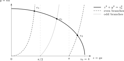
Graphical root construction for $z_0=4$. The quarter circle intersects two even branches and one odd branch, giving three bound states. Dashed vertical guides mark the parity-branch boundaries at $\pi/2$ and $\pi$; tangent poles are clipped.

Worked Example: Strength Four

For $z_0=4$, bracketed root solving gives:

State	Parity	$z=qa$	$y=\kappa a$	$E/V_0$	$P_{\mathrm{out}}$
1	even	$1.2524$	$3.7989$	$-0.9020$	$0.0204$
2	odd	$2.4746$	$3.1427$	$-0.6173$	$0.0924$
3	even	$3.5953$	$1.7532$	$-0.1921$	$0.2934$

The parity alternates and the node count increases with energy. The highest state is closest to threshold, has the smallest decay constant, and places nearly thirty percent of its probability outside the nominal well. Finite confinement is therefore not a small boundary correction for weakly bound levels.

Number Of Bound States

As $V_0$, $a$, or $m$ increases, $z_0$ increases and more bound states fit inside the well. There is always at least one even bound state for an attractive one-dimensional finite square well. Additional states appear as the well becomes deeper or wider.

For this width and strength convention, the exact count is

$$N_{\mathrm{bound}} =\left\lceil\frac{2z_0}{\pi}\right\rceil, \qquad z_0\gt0.$$

To see the threshold convention, suppose $z_0=r\pi/2$ for a positive integer $r$. The candidate next state then has $y=\kappa a=0$ and sits at $E=0$, so its exterior wavefunction does not decay and it is not normalizable. The ceiling formula counts only the $r$ states already below threshold. Immediately above that value of $z_0$, a new bound level appears.

Equivalent formulas using a floor function must state how exact thresholds are handled. They also often define the width parameter as $2a$, so copying a count without checking conventions can introduce a factor of two.

The broader counting logic, including threshold caveats and semiclassical scaling, is collected in Bound-State Counting.

Shallow-Well Limit

When $z_0\ll1$, only the even ground state exists. Its root has $z\ll1$ and $y\ll1$. The even equation and circle give, to leading order,

$$y=z\tan z\simeq z^2, \qquad z^2+y^2=z_0^2,$$

so $z\simeq z_0$ and $y\simeq z_0^2$. The binding energy is therefore

$$E =-\frac{\hbar^2\kappa^2}{2m} \simeq -\frac{2mV_0^2a^2}{\hbar^2}.$$

The energy is quadratic in the weak well strength, while the tail length scales as $1/\kappa\sim a/z_0^2$ and becomes much larger than the well. This explicit limit realizes the general one-dimensional result that an arbitrarily weak attractive potential supports at least one bound state.

Infinite-Well Limit

As $V_0\to\infty$, the decay constant $\kappa$ becomes large and the exterior tails shrink. The wavefunction becomes effectively zero at $x=\pm a$, and the finite-well spectrum approaches the infinite-well spectrum on an interval of length $2a$:

$$E_n^{\text{inside}} \sim \frac{n^2\pi^2\hbar^2}{2m(2a)^2},$$

measured upward from the bottom of the well. The total energy relative to the outside zero is shifted by approximately $-V_0$.

More explicitly, at fixed level index,

$$z_n\longrightarrow\frac{n\pi}{2}$$

from below, and

$$E_n =-V_0+\frac{\hbar^2z_n^2}{2ma^2} \longrightarrow -V_0+\frac{n^2\pi^2\hbar^2}{8ma^2}.$$

The total energies tend to $-\infty$ under the exterior-zero convention because the well bottom is moving downward. The finite excitation energies $E_n+V_0$ are what approach the infinite-well spectrum. Keeping the energy zero fixed is essential when taking this limit.

The finite well therefore explains why the infinite well is an idealization: real finite confinement has penetration depth.

Physical Interpretation

Outside the well, the bound-state wavefunction decays as

$$e^{-\kappa \lvert x\rvert}.$$

The decay length is

$$\ell_{\text{tail}}=\frac{1}{\kappa}.$$

A state close to threshold has small $\kappa$ and a long tail. A deeply bound state has larger $\kappa$ and is more tightly localized. This tail behavior is a first encounter with tunneling: the wavefunction can enter a classically forbidden region, even though a bound-state probability density remains normalizable.

An evanescent tail does not mean that a stationary bound state is steadily leaking away. The parity eigenfunctions can be chosen real, so their probability current vanishes everywhere. Their exterior probability is time independent. Escape requires coupling to an open channel, a time-dependent perturbation, or a potential for which the state is a resonance rather than a true bound eigenstate.

Ordering, Parity, and Nodes

One-dimensional bound levels are nondegenerate. For this symmetric well they alternate in parity:

$$\text{even ground state}, \quad \text{odd first excited state}, \quad \text{even second excited state}, \quad\ldots$$

Ordered by increasing energy, the $n$th bound state has $n-1$ nodes. The ground state is everywhere of one sign, the first odd state has its node at the origin, and each subsequent branch adds one interior node. This ordering is a consequence of the one-dimensional oscillation theorem, not a peculiarity of square wells.

Bound and Continuum Sectors

The finite set of bound eigenfunctions is not complete by itself. The full spectral resolution also contains continuum scattering states. Schematically,

$$\hat I =\sum_{n\in\mathrm{bound}} |n\rangle\langle n| +\sum_{s=e,o} \int_0^\infty dE\, |E,s\rangle\langle E,s|,$$

where the continuum normalization convention must be specified. A localized initial state can have projections onto both sectors: the bound component remains near the well, while the continuum component disperses to infinity.

At $E=0$, the exterior solution is constant or linear rather than exponentially decaying. A specially tuned threshold solution can strongly influence low-energy scattering, but it is not an ordinary $L^2$ bound state in this one-dimensional problem.

Reliable Numerical Root Finding

For a given $z_0$, solve separately in each allowed parity interval truncated at $z=z_0$. Define

$$\begin{aligned} f_e(z) &=z\tan z-\sqrt{z_0^2-z^2},\\ f_o(z) &=-z\cot z-\sqrt{z_0^2-z^2}. \end{aligned}$$

A bracketing method such as bisection or Brent’s method is safer than an unrestricted Newton iteration because tangent and cotangent have poles. Do not let a bracket cross a pole, and exclude a root with $z=z_0$ because it has $\kappa=0$.

After finding $z$, reconstruct

$$q=\frac{z}{a}, \qquad \kappa=\frac{\sqrt{z_0^2-z^2}}{a}, \qquad E=V_0\left(\frac{z^2}{z_0^2}-1\right).$$

Then verify the original matching equations, normalize the piecewise state, and check that $\psi$ and $\psi'$ agree at both interfaces. A direct finite-difference diagonalization on a sufficiently large exterior domain should converge to the same negative energies, but its box size must be several tail lengths for the least-bound state.

Common Mistakes

• Setting $\psi(\pm a)=0$ for a finite well.
• Forgetting evanescent tails outside the well.
• Interpreting a stationary evanescent tail as a probability current leaking to infinity.
• Mixing the even equation $q\tan(qa)=\kappa$ with the odd equation $-q\cot(qa)=\kappa$.
• Treating the transcendental equations as if every mathematical root were physically allowed without checking $-V_0\lt E\lt0$.
• Counting an $E=0$ threshold solution as a normalizable bound state.
• Using a floor-function state count without checking the width convention and exact-threshold rule.
• Measuring energies inconsistently, sometimes from the well bottom and sometimes from the outside zero.
• Assuming the finite-well spectrum has the same $n^2$ spacing as the infinite well.
• Solving across tangent poles with an unbracketed root finder and accepting a discontinuity as a zero.
• Normalizing only inside the well and omitting the exterior probability.
• Treating the finite list of bound states as a complete basis without the continuum sector.

Where This Is Used

• Infinite Square Well is the infinite-depth limit.
• Energy Scales in One Dimension explains the $z_0$ strength parameter and tail-length scale.
• Bound-State Counting explains how graphical finite-well roots translate into a state count.
• Parity and Nodes explains why the finite well separates into even and odd sectors.
• Boundary Conditions explains continuity and derivative matching at finite jumps.
• Normalization Conventions distinguishes bound-state and continuum normalization.
• Probability Current explains why real stationary tails do not represent leakage.
• Matrix Diagonalization gives numerical tools for finding finite-well spectra.
• Sturm–Liouville Theory explains the eigenvalue-problem structure.
• Quantum Wells adds material-dependent effective masses, heterointerface matching, in-plane subbands, self-consistent electrostatics, and optical transitions.
• Rectangular Barrier Tunneling reuses evanescent waves in an open scattering problem.

References

• D. J. Griffiths and D. F. Schroeter, Introduction to Quantum Mechanics, 3rd ed., Cambridge University Press, 2018.
• R. Shankar, Principles of Quantum Mechanics, 2nd ed., Springer, 1994.
• C. Cohen-Tannoudji, B. Diu, and F. Laloë, Quantum Mechanics, Wiley, 1977.
• E. Merzbacher, Quantum Mechanics, 3rd ed., Wiley, 1998.
• L. D. Landau and E. M. Lifshitz, Quantum Mechanics: Non-Relativistic Theory, 3rd ed., Butterworth-Heinemann, 1977.

Exercises

1. Derive the even-state equation $q\tan(qa)=\kappa$ from continuity of $\psi$ and $\psi'$ at $x=a$.

Solution

For the even state,

$$\psi(x)=A\cos(qx)$$

inside and

$$\psi(x)=B e^{-\kappa x}$$

for $x\gt a$. Matching values at $a$ gives

$$A\cos(qa)=B e^{-\kappa a}.$$

Matching derivatives gives

$$-Aq\sin(qa)=-B\kappa e^{-\kappa a}.$$

Divide the derivative equation by the value equation:

$$\frac{q\sin(qa)}{\cos(qa)}=\kappa,$$

so $q\tan(qa)=\kappa$.

2. Explain why a state with $E\gt0$ is not a bound state for the convention used on this page.

Solution

Outside the well, $V=0$. If $E\gt0$, the outside Schrödinger equation has oscillatory solutions rather than decaying exponentials. Such states are scattering states, not square-normalizable bound states.

3. What happens to the tail length as a bound-state energy approaches $E=0$ from below? Does the growing tail imply a nonzero outward probability current for a stationary parity eigenstate?

Solution

The outside decay constant is

$$\kappa=\frac{\sqrt{-2mE}}{\hbar}.$$

As $E\to 0^-$, $\kappa\to 0$, so the tail length $1/\kappa$ diverges. The state becomes weakly bound and spatially extended.

The state can be chosen real, apart from its common factor $e^{-iEt/\hbar}$. Therefore

$$j=\frac{\hbar}{m}\operatorname{Im}(\psi^*\psi')=0.$$

The exterior probability is stationary; a long tail is not a decay flux.

4. Derive the even-state normalization constant and its exterior probability using the interface-anchored wavefunction.

Solution

By parity,

$$\begin{aligned} 1 &=2\mathcal N_e^2 \left[ \int_0^a\cos^2(qx)\,dx +\cos^2(qa) \int_a^\infty e^{-2\kappa(x-a)}\,dx \right]\\ &=\mathcal N_e^2 \left[ a+\frac{\sin(2qa)}{2q} +\frac{\cos^2(qa)}{\kappa} \right]. \end{aligned}$$

Hence

$$\mathcal N_e^{-2} =a+\frac{\sin(2qa)}{2q} +\frac{\cos^2(qa)}{\kappa}.$$

The two exterior tails contribute

$$P_{\mathrm{out}} =2\mathcal N_e^2\cos^2(qa) \int_a^\infty e^{-2\kappa(x-a)}\,dx =\frac{\mathcal N_e^2\cos^2(qa)}{\kappa}.$$

5. Use $N_{\mathrm{bound}}=\lceil2z_0/\pi\rceil$ to count the bound states at $z_0=0.8$, $z_0=\pi/2$, $z_0=\pi/2+0.1$, $z_0=\pi$, and $z_0=\pi+0.1$. Explain the values at exact thresholds.

Solution

The counts are

$$\begin{array}{c|ccccc} z_0 & 0.8 & \pi/2 & \pi/2+0.1 & \pi & \pi+0.1\\ \hline N_{\mathrm{bound}} & 1 & 1 & 2 & 2 & 3. \end{array}$$

At $z_0=\pi/2$, the candidate odd state has just reached $E=0$ and is not normalizable, so only the even ground state is bound. Just above the threshold, that odd state moves below zero. The same logic applies to the candidate second even state at $z_0=\pi$.

6. Derive the leading shallow-well binding energy for $z_0\ll1$ and compare it with the bound energy of an attractive delta potential having the same integrated strength.

Solution

For the even ground state,

$$y=z\tan z\simeq z^2.$$

The circle relation $z^2+y^2=z_0^2$ then gives $z\simeq z_0$ and $y\simeq z_0^2$. Since $\kappa=y/a$,

$$E =-\frac{\hbar^2\kappa^2}{2m} \simeq -\frac{\hbar^2z_0^4}{2ma^2} =-\frac{2mV_0^2a^2}{\hbar^2}.$$

The integrated attractive strength is

$$g=\int_{-a}^{a}V_0\,dx=2aV_0.$$

An attractive potential $-g\delta(x)$ has bound energy $-mg^2/(2\hbar^2)$, which becomes

$$-\frac{m(2aV_0)^2}{2\hbar^2} =-\frac{2mV_0^2a^2}{\hbar^2}.$$

The agreement reflects the fact that a sufficiently narrow or weak well is controlled at leading order by its integrated attraction.