Square-Well Scattering

Here “square well” means an attractive spherical well in three spatial dimensions, not the one-dimensional finite well. The distinction matters: this calculation is organized by angular-momentum channels, phase shifts, and cross sections.

The model is elementary enough to solve exactly but rich enough to display three central scattering ideas:

• interface matching determines every partial-wave phase shift;
• the zero-energy $s$-wave solution determines the scattering length;
• a centrifugal barrier can turn an almost-bound higher-partial-wave state into a shape resonance.

Phase Shifts owns the general interpretation of $\delta_\ell$, Scattering Length owns the threshold parameter, and Resonances owns the general resonance classification. This page carries one fixed model through all three structures.

Problem Statement

Consider relative motion with reduced mass $\mu$ in

$$V(r) = \begin{cases} -V_0, & 0\le r<R, \\ 0, & r>R, \end{cases} \qquad V_0\gt0.$$

For positive scattering energy,

$$E = \frac{\hbar^2k^2}{2\mu}, \qquad k\gt0,$$

the interior wave number is

$$q = \frac{\sqrt{2\mu(E+V_0)}}{\hbar}.$$

The tasks are to:

1. derive the exact elastic phase shift $\delta_\ell(k)$ for every partial wave;
2. recover the exact $s$-wave scattering length;
3. identify threshold and shape-resonance behavior;
4. check unitarity, weak coupling, and the zero-energy limit.

No approximation is needed for the matching calculation. Approximations enter only when the exact answer is reduced to a low-energy or weak-coupling form.

Dimensionless Control Parameters

Use the range $R$ to define

$$x=kR, \qquad y=qR, \qquad g = \frac{R\sqrt{2\mu V_0}}{\hbar}.$$

These variables satisfy

$$y=\sqrt{x^2+g^2}.$$

The dimensionless depth $g^2$ compares the well depth with

$$E_R = \frac{\hbar^2}{2\mu R^2},$$

because

$$\frac{V_0}{E_R}=g^2.$$

Thus:

• $x$ controls the incident wavelength relative to the range;
• $g$ controls the interaction strength and the number of bound states;
• $y$ is the interior phase accumulated over one radius.

The low-energy regime is $x\ll1$. It is not the same as weak coupling: $g$ may be tuned arbitrarily close to a threshold state while $x$ remains small.

Exact Partial-Wave Matching

Write the wavefunction as

$$\psi(\mathbf r) = \sum_{\ell,m} \frac{u_\ell(r)}{r} Y_{\ell m}(\widehat{\mathbf r}).$$

The reduced radial equation is

$$\begin{aligned} - \frac{\hbar^2}{2\mu} \frac{d^2u_\ell}{dr^2} + V(r)u_\ell(r) \\ + \frac{\hbar^2\ell(\ell+1)}{2\mu r^2} u_\ell(r) &= E u_\ell(r). \end{aligned}$$

Regularity at the origin requires

$$u_\ell(r)\propto r^{\ell+1} \qquad (r\to0).$$

Introduce the Riccati–Bessel functions

$$\widehat j_\ell(z)=zj_\ell(z), \qquad \widehat n_\ell(z)=zn_\ell(z).$$

Their definitions and recurrences are collected in Bessel Functions.

Interior solution

The regular interior solution is

$$u_\ell^{\mathrm{in}}(r) = A_\ell\widehat j_\ell(qr).$$

The irregular Riccati–Neumann solution is excluded at the origin.

Exterior solution

Choose the real standing-wave convention

$$\begin{aligned} u_\ell^{\mathrm{out}}(r) ={}& B_\ell \left[ \widehat j_\ell(kr)\cos\delta_\ell \right. \\ &\left. - \widehat n_\ell(kr)\sin\delta_\ell \right]. \end{aligned}$$

At large $r$ this becomes

$$u_\ell^{\mathrm{out}}(r) \sim B_\ell \sin\left( kr-\frac{\ell\pi}{2}+\delta_\ell \right).$$

This fixes the sign convention for $\delta_\ell$.

Match logarithmic derivatives

Because the potential step is finite, both $u_\ell$ and $u_\ell'$ are continuous at $r=R$. The overall normalization cancels if one matches the logarithmic derivative.

Define

$$\mathcal L_\ell = \frac{ \left.u_\ell^{\mathrm{in}\,\prime}(r)\right|_{R} }{ u_\ell^{\mathrm{in}}(R) } = q \frac{ \widehat j_\ell'(y) }{ \widehat j_\ell(y) },$$

where a prime on a Riccati–Bessel function means differentiation with respect to its argument.

At the boundary, abbreviate

$$\begin{aligned} J_\ell&=\widehat j_\ell(x), & N_\ell&=\widehat n_\ell(x), \\ J_\ell'&=\widehat j_\ell'(x), & N_\ell'&=\widehat n_\ell'(x). \end{aligned}$$

Matching gives

$$\frac{\mathcal L_\ell}{k} = \frac{ J_\ell'\cos\delta_\ell - N_\ell'\sin\delta_\ell }{ J_\ell\cos\delta_\ell - N_\ell\sin\delta_\ell }.$$

Solving for the phase shift,

$$\tan\delta_\ell = \frac{ kJ_\ell'-\mathcal L_\ell J_\ell }{ kN_\ell'-\mathcal L_\ell N_\ell }.$$

It is convenient to define

$$\lambda_\ell = \frac{\mathcal L_\ell}{k} = \frac{y}{x} \frac{ \widehat j_\ell'(y) }{ \widehat j_\ell(y) },$$

so the same result is

$$\tan\delta_\ell = \frac{ J_\ell'-\lambda_\ell J_\ell }{ N_\ell'-\lambda_\ell N_\ell }.$$

This is the exact answer for every $\ell$.

Branch handling

The tangent determines $\delta_\ell$ only modulo $\pi$. A numerical calculation should evaluate

$$\delta_\ell = \operatorname{atan2} \left( J_\ell'-\lambda_\ell J_\ell,\, N_\ell'-\lambda_\ell N_\ell \right)$$

and then unwrap the result continuously in $k$ or in the well depth. Using a one-argument arctangent can manufacture discontinuities or erase the phase motion through a resonance.

The branch choice does not affect $\sin^2\delta_\ell$, but it matters for Levinson-theorem checks and for distinguishing rapid resonant motion from a plotting artifact.

S-Wave Formula

For $\ell=0$,

$$\widehat j_0(z)=\sin z, \qquad \widehat n_0(z)=-\cos z.$$

The interior and exterior solutions can therefore be written as

$$u_0^{\mathrm{in}}(r)=A\sin(qr),$$

and

$$u_0^{\mathrm{out}}(r)=B\sin(kr+\delta_0).$$

Logarithmic-derivative matching gives

$$q\cot(qR) = k\cot(kR+\delta_0),$$

or

$$\tan(x+\delta_0) = \frac{x}{y}\tan y.$$

Eliminating the sum angle gives the explicit tangent

$$\tan\delta_0 = \frac{ x\tan y-y\tan x }{ y+x\tan y\tan x }.$$

This expression is useful for threshold expansions. Near poles of either tangent, the logarithmic-derivative or two-argument form is numerically safer.

Unitarity and Cross Sections

For a real well with no open inelastic channel, every exact phase shift is real. Hence

$$S_\ell=e^{2i\delta_\ell}$$

satisfies

$$|S_\ell|=1.$$

The partial-wave amplitude is

$$f_\ell(k) = \frac{ e^{2i\delta_\ell}-1 }{ 2ik } = \frac{ e^{i\delta_\ell}\sin\delta_\ell }{k},$$

and the elastic partial cross section is

$$\sigma_\ell = \frac{4\pi}{k^2} (2\ell+1) \sin^2\delta_\ell.$$

Each channel obeys the elastic unitarity bound

$$\sigma_\ell \le \frac{4\pi}{k^2}(2\ell+1).$$

For ordinary short-range scattering away from a threshold anomaly,

$$\delta_\ell=O\left(k^{2\ell+1}\right).$$

The centrifugal barrier therefore suppresses higher partial waves at low energy. A near-threshold shape resonance is an important exception over a narrow energy interval.

Exact S-Wave Scattering Length

At zero energy, the regular interior solution is

$$u_0^{\mathrm{in}}(r) = A\sin\left( \frac{g r}{R} \right).$$

Outside the finite-range interaction, the general zero-energy $s$-wave solution is linear:

$$u_0^{\mathrm{out}}(r)=B(r-a_s),$$

where $a_s$ is the scattering length.

Matching logarithmic derivatives at $R$ gives

$$\frac{g}{R}\cot g = \frac{1}{R-a_s}.$$

Therefore

$$\frac{a_s}{R} = 1-\frac{\tan g}{g}.$$

This exact result is the threshold fingerprint of the whole well.

Weak-coupling check

For $g\ll1$,

$$\frac{\tan g}{g} = 1+\frac{g^2}{3} +\frac{2g^4}{15} +O(g^6),$$

so

$$\frac{a_s}{R} = - \frac{g^2}{3} - \frac{2g^4}{15} +O(g^6).$$

The first Born scattering length is

$$a_s^{(1)} = \frac{2\mu}{\hbar^2} \int_0^\infty r^2V(r)\,dr.$$

For the attractive square well,

$$a_s^{(1)} = - \frac{2\mu V_0R^3}{3\hbar^2} = - \frac{g^2R}{3},$$

which agrees with the leading exact term. Validity of the Born Approximation uses the same comparison to show why the smooth weak-coupling expansion cannot reproduce a threshold pole.

Bound-state thresholds

The scattering length diverges when

$$\cos g=0,$$

that is,

$$g = \left( n+\frac12 \right)\pi, \qquad n=0,1,2,\ldots.$$

At each such depth, an $s$-wave state sits at zero energy. As the well is deepened through the threshold, the pole moves between a virtual-state continuation and a normalizable bound state, while $a_s$ jumps through infinity.

The divergence is not a failure of the exact solution. It is the physical signal that the low-energy amplitude has become nonperturbative.

Low-energy cross section

Keeping only the scattering length,

$$f_0(k) \approx - \frac{a_s}{1+ika_s},$$

so

$$\sigma_0(k) \approx \frac{ 4\pi a_s^2 }{ 1+k^2a_s^2 }.$$

If $k|a_s|\ll1$, this reduces to

$$\sigma_0\approx4\pi a_s^2.$$

If $|a_s|\to\infty$ at fixed nonzero $k$, the cross section instead approaches

$$\sigma_0\to\frac{4\pi}{k^2}.$$

The order of limits matters. Setting $k=0$ before tuning $a_s$ to infinity hides the finite-energy unitarity bound.

Shape Resonance in the P Wave

The effective radial potential is

$$V_{\mathrm{eff},\ell}(r) = V(r) + \frac{ \hbar^2\ell(\ell+1) }{ 2\mu r^2 }.$$

For $\ell\ge1$, the attractive interior is separated from infinity by a centrifugal barrier. A state that would be bound in a slightly deeper well can then remain temporarily localized and leak through the barrier. This is a shape resonance.

First p-wave threshold

At zero energy, a normalizable $\ell=1$ exterior solution behaves as

$$u_1^{\mathrm{out}}(r)\propto r^{-1}.$$

Its logarithmic derivative at $R$ is $-1/R$. The interior threshold condition is therefore

$$g \frac{ \widehat j_1'(g) }{ \widehat j_1(g) } = -1.$$

Use the recurrence

$$\widehat j_1'(g) = \widehat j_0(g) - \frac{1}{g}\widehat j_1(g).$$

The threshold condition reduces to

$$\widehat j_0(g)=\sin g=0.$$

The first $p$-wave bound state therefore reaches threshold at

$$g=\pi.$$

For a depth slightly below this value, the state lies in the continuum but remains trapped behind the centrifugal barrier long enough to generate rapid phase motion.

Concrete resonance audit

Choose

$$g=3.13,$$

which is just below $\pi$. Evaluating the exact matching formula gives a low-energy $p$-wave peak at

$$x_r=k_rR\approx0.1568,$$

where

$$\sin^2\delta_1(x_r)\approx1.$$

The $p$-wave cross section therefore reaches its elastic unitarity limit:

$$\begin{aligned} \frac{\sigma_1(x_r)}{\pi R^2} &= \frac{12}{x_r^2} \sin^2\delta_1(x_r) \\ &\approx 488.1. \end{aligned}$$

The half-maximum points of $\sin^2\delta_1$ occur at

$$x_-\approx0.14942, \qquad x_+\approx0.16636.$$

These numbers diagnose a localized phase-shift feature. They are not yet a Breit–Wigner energy width: a proper resonance fit must use energy rather than $x$, retain the background phase, and test whether a single isolated pole controls the interval. Resonance from a Square Well performs that fit and compares it with the exact outgoing-wave pole.

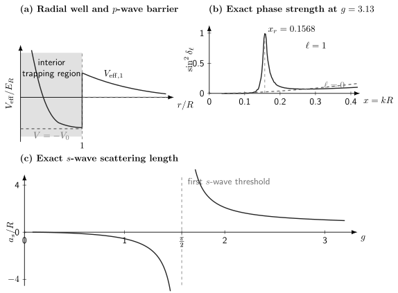
Top left: the square well and the $\ell=1$ effective potential create a trapping region behind a centrifugal barrier. Top right: at $g=3.13$, just below the first $p$-wave threshold $g=\pi$, the exact $\sin^2\delta_1$ develops a narrow low-energy peak while the $s$ wave varies smoothly. Bottom: $a_s/R=1-\tan g/g$ diverges when the first $s$-wave state reaches threshold at $g=\pi/2$.

Threshold Convergence Check

For the same $g=3.13$, the exact zero-energy formula gives

$$\frac{a_s}{R} = 1-\frac{\tan(3.13)}{3.13} \approx 1.003703889.$$

At finite $x$, extract an effective estimate from the exact phase shift:

$$\frac{a_s(x)}{R} = - \frac{\tan\delta_0(x)}{x}.$$

The result converges quadratically toward the zero-energy value.

$x=kR$	$a_s(x)/R$	Relative difference from $a_s/R$
$0.20$	$1.015279514$	$1.15\times10^{-2}$
$0.10$	$1.006570923$	$2.86\times10^{-3}$
$0.05$	$1.004418987$	$7.12\times10^{-4}$
$0.02$	$1.003818231$	$1.14\times10^{-4}$
$0.01$	$1.003732472$	$2.85\times10^{-5}$

The factor-of-four reduction in error whenever $x$ is halved is consistent with the first omitted effective-range correction being $O(x^2)$.

At $x=0.05$, the exact $s$-wave cross section is

$$\frac{\sigma_0}{\pi R^2} = \frac{4\sin^2\delta_0}{x^2} \approx 4.0253,$$

close to the strict threshold prediction

$$\frac{4a_s^2}{R^2} \approx 4.0297.$$

This check probes the finite-$k$ approach to the zero-energy formula independently of the algebra used to solve for $a_s$ directly.

Interpretation

The same well depth organizes different physical phenomena in different angular-momentum channels.

For the $s$ wave, no centrifugal barrier exists. Tuning through $g=(n+1/2)\pi$ moves a pole through zero energy and makes the scattering length diverge. The resulting enhancement is a threshold phenomenon rather than a long-lived shape resonance behind a barrier.

For $\ell\ge1$, the centrifugal term supplies a barrier. A near-threshold level can remain quasibound at positive energy and produce a sharp phase-shift feature. The feature narrows as the level approaches threshold because penetration through the barrier is increasingly suppressed.

At higher energy, more partial waves contribute. A useful geometric estimate is

$$\ell_{\max}\sim kR=x,$$

because channels with impact parameter substantially larger than the range barely sample the interaction.

Validity and Scope

The calculation is exact under the stated assumptions:

• nonrelativistic two-body relative motion;
• a central, real, energy-independent potential;
• one elastic channel;
• a sharp spherical step of radius $R$;
• no spin, tensor force, spin–orbit coupling, or absorption.

Using the square well as a model of a microscopic interaction is a separate approximation. Its threshold observables may be useful at wavelengths much longer than $R$, but detailed high-energy phase shifts are sensitive to the unphysical discontinuity at the boundary.

Near a resonance, tiny changes in $g$ can move the peak substantially. Quoting a resonance location without the depth convention, radius, branch handling, and numerical resolution is not reproducible.

Common Mistakes

• Using the one-dimensional finite-well matching formulas for a spherical scattering problem.
• Matching the radial function $R_\ell(r)$ as though it were the reduced function $u_\ell(r)=rR_\ell(r)$.
• Keeping the irregular Riccati–Neumann solution at the origin.
• Forgetting that primes on $\widehat j_\ell$ and $\widehat n_\ell$ differentiate their arguments, producing factors of $q$ or $k$ in radial derivatives.
• Computing $\delta_\ell$ with a one-argument arctangent and interpreting branch jumps as resonances.
• Calling every point with $\sin^2\delta_\ell=1$ a narrow resonance without checking phase motion, background, and width.
• Treating low energy as synonymous with weak scattering near a threshold pole.
• Applying $\sigma_0\approx4\pi a_s^2$ when $k|a_s|$ is not small.
• Forgetting the factor $2\ell+1$ in the partial-wave cross section.

Exercises

1. Derive the matching formula

Starting from continuity of the logarithmic derivative, derive

$$\tan\delta_\ell = \frac{ kJ_\ell'-\mathcal L_\ell J_\ell }{ kN_\ell'-\mathcal L_\ell N_\ell }.$$

Solution

At $r=R$,

$$\mathcal L_\ell = k \frac{ J_\ell'\cos\delta_\ell - N_\ell'\sin\delta_\ell }{ J_\ell\cos\delta_\ell - N_\ell\sin\delta_\ell }.$$

Cross-multiplication gives

$$\begin{aligned} \mathcal L_\ell J_\ell\cos\delta_\ell &- \mathcal L_\ell N_\ell\sin\delta_\ell \\ &= kJ_\ell'\cos\delta_\ell - kN_\ell'\sin\delta_\ell. \end{aligned}$$

Move the cosine terms to one side and the sine terms to the other:

$$\begin{aligned} & \left( kN_\ell'-\mathcal L_\ell N_\ell \right) \sin\delta_\ell \\ &\qquad = \left( kJ_\ell'-\mathcal L_\ell J_\ell \right) \cos\delta_\ell. \end{aligned}$$

Division by the cosine coefficient gives the stated tangent whenever that representation is finite. The two-argument arctangent covers the exceptional points.

2. Check the zero-potential limit

Set $V_0=0$, so $q=k$ and $y=x$. Show that every phase shift vanishes modulo $\pi$.

Solution

When $q=k$,

$$\mathcal L_\ell = k \frac{J_\ell'}{J_\ell}.$$

The numerator of the exact tangent becomes

$$kJ_\ell' - \mathcal L_\ell J_\ell = kJ_\ell' - k\frac{J_\ell'}{J_\ell}J_\ell = 0.$$

Thus $\tan\delta_\ell=0$. Choosing the branch continuously connected to free motion gives

$$\delta_\ell=0.$$

Consequently $S_\ell=1$ and every scattering cross section vanishes.

3. Derive the scattering length

Match the zero-energy solutions and derive

$$\frac{a_s}{R} = 1-\frac{\tan g}{g}.$$

Solution

The interior and exterior logarithmic derivatives at $R$ are

$$\left. \frac{u_{\mathrm{in}}'}{u_{\mathrm{in}}} \right|_R = \frac{g}{R}\cot g,$$

and

$$\left. \frac{u_{\mathrm{out}}'}{u_{\mathrm{out}}} \right|_R = \frac{1}{R-a_s}.$$

Equating them,

$$R-a_s = \frac{R}{g\cot g} = R\frac{\tan g}{g}.$$

Therefore

$$a_s = R \left( 1-\frac{\tan g}{g} \right).$$

4. Compare with the Born approximation

Expand the exact scattering length through $O(g^4)$ and verify its leading term from the first Born formula.

Solution

The tangent expansion is

$$\tan g = g+\frac{g^3}{3} +\frac{2g^5}{15} +O(g^7).$$

Hence

$$\frac{a_s}{R} = - \frac{g^2}{3} - \frac{2g^4}{15} +O(g^6).$$

The first Born result is

$$\begin{aligned} a_s^{(1)} &= \frac{2\mu}{\hbar^2} \int_0^R r^2(-V_0)\,dr \\ &= - \frac{2\mu V_0R^3}{3\hbar^2} \\ &= - \frac{g^2R}{3}. \end{aligned}$$

It reproduces the leading exact term but cannot produce the poles at finite $g$.

5. Locate the s-wave threshold states

Explain why $a_s$ diverges at $g=(n+1/2)\pi$ and connect this condition with a zero-energy state.

Solution

The divergence occurs when $\tan g$ has a pole:

$$\cos g=0.$$

At $a_s=\infty$, the normalized zero-energy exterior form $u_{\mathrm{out}}\propto r-a_s$ can be rescaled to approach a constant. Its logarithmic derivative at the boundary therefore tends to zero.

The interior logarithmic derivative must also vanish:

$$\frac{g}{R}\cot g=0.$$

For nonzero $g$, this requires $\cot g=0$, which gives

$$g = \left( n+\frac12 \right)\pi.$$

This is precisely the condition for an $s$-wave level at threshold.

6. Locate the first p-wave threshold

Use the zero-energy exterior behavior and a Riccati–Bessel recurrence to show that the first $p$-wave bound state reaches threshold at $g=\pi$.

Solution

For $\ell=1$, the normalizable zero-energy exterior solution is

$$u_1(r)\propto r^{-1},$$

so

$$\left. R\frac{u_1'}{u_1} \right|_R = -1.$$

The interior solution is $\widehat j_1(gr/R)$, giving

$$g \frac{ \widehat j_1'(g) }{ \widehat j_1(g) } = -1.$$

Using

$$\widehat j_1'(g) = \widehat j_0(g) - \frac{\widehat j_1(g)}{g},$$

the left side becomes

$$g \frac{ \widehat j_0(g) }{ \widehat j_1(g) } -1.$$

Equating this to $-1$ requires

$$\widehat j_0(g)=\sin g=0.$$

The first positive solution is $g=\pi$. A well with $g$ just below $\pi$ can therefore support a near-threshold $p$-wave shape resonance without yet supporting the corresponding bound state.

Cross-Links

• Radial Schrödinger Equation
• Partial-Wave Expansion
• Phase Shifts
• Partial-Wave Cross Sections
• Scattering Length
• Low-Energy Scattering
• Low-Energy S-Wave Scattering
• Resonance from a Square Well
• Resonances
• Bound States and Scattering Poles
• Validity of the Born Approximation
• Phase Shift Extraction Notebook
• Finite Square Well

References

• J. R. Taylor, Scattering Theory: The Quantum Theory of Nonrelativistic Collisions, Dover, 2006.
• R. G. Newton, Scattering Theory of Waves and Particles, 2nd ed., Dover, 2002.
• C. J. Joachain, Quantum Collision Theory, 3rd ed., North-Holland, 1983.
• L. D. Landau and E. M. Lifshitz, Quantum Mechanics: Non-Relativistic Theory, 3rd ed., Pergamon, 1977.
• A. Messiah, Quantum Mechanics, Vol. I, North-Holland, 1961.