Low-Energy S-Wave Scattering

This worked problem turns low-energy universality into a quantitative approximation test. An attractive spherical square well is tuned to have a scattering length ten times its range. The exact $s$-wave solution is then compared with:

1. the scattering-length amplitude;
2. the effective-range approximation;
3. the $s$-wave unitarity bound;
4. the exact shallow-bound-state pole.

The point is not that a square well is a realistic microscopic interaction. It is that one exactly solvable short-range model makes every scale and every omitted term visible. Low-Energy Scattering owns the general universality statement, while Square-Well Scattering owns the full finite-energy matching problem in all partial waves.

Problem Statement

Consider relative motion with reduced mass $\mu$ in

$$V(r) = \begin{cases} -V_0, & 0\le r<R, \\ 0, & r>R, \end{cases} \qquad V_0>0.$$

Define the range energy and dimensionless variables

$$\begin{aligned} E_R &= \frac{\hbar^2}{2\mu R^2}, \\ x &= kR, \\ g &= \frac{R\sqrt{2\mu V_0}}{\hbar}. \end{aligned}$$

The well depth is $V_0/E_R=g^2$. At positive collision energy,

$$E = \frac{\hbar^2k^2}{2\mu},$$

the interior wave number $q$ obeys

$$y \equiv qR = \sqrt{g^2+x^2}.$$

The target is the elastic $s$-wave cross section for distinguishable particles. Identical-particle factors are discussed separately below.

Method Choice

The calculation uses the exact square-well phase shift as an independent benchmark. It then deliberately discards short-distance information in stages:

$$\begin{gathered} K_{\mathrm{exact}}(k) \equiv k\cot\delta_0(k), \\ K_{\mathrm{ERE}}(k) = -\frac1a + \frac12r_e k^2, \\ K_{\mathrm{univ}}(k) = -\frac1a. \end{gathered}$$

All three are inserted into the same unitary amplitude

$$f_0(k) = \frac{1}{K(k)-ik}.$$

This comparison separates two issues that are often mixed together:

• keeping the exact unitarity denominator $-ik$;
• approximating the real short-range function $K(k)=k\cot\delta_0(k)$.

The scattering-length approximation is nonperturbative in $ka$ even though it is the leading term in an expansion in the interaction range.

Exact S-Wave Input

For the regular reduced radial wavefunction,

$$\begin{aligned} u_0^{\mathrm{in}}(r) &\propto \sin(qr), \\ u_0^{\mathrm{out}}(r) &\propto \sin(kr+\delta_0). \end{aligned}$$

Matching logarithmic derivatives at $r=R$ gives

$$y\cot y = x\cot(x+\delta_0).$$

It is convenient to define

$$T(x) = \frac{x}{y}\tan y.$$

The matching condition becomes

$$\tan(x+\delta_0) = T(x).$$

Using the tangent subtraction identity gives an exact expression without choosing a phase branch:

$$\tan\delta_0 = \frac{T(x)-\tan x} {1+T(x)\tan x}.$$

Therefore the exact dimensionless effective-range function is

$$\mathcal K_{\mathrm{exact}}(x) \equiv x\cot\delta_0 = x \frac{1+T(x)\tan x} {T(x)-\tan x}.$$

No inverse tangent appears, so this formula is continuous through points where $\delta_0$ crosses $\pi/2$.

Tune a Large Scattering Length

The exact square-well scattering length is

$$a = R\left( 1-\frac{\tan g}{g} \right).$$

Write

$$A \equiv \frac{a}{R}.$$

The benchmark is chosen by imposing

$$A=10.$$

The first solution above the one-bound-state threshold $g=\pi/2$ is

$$g = 1.63850515464009.$$

It satisfies

$$1-\frac{\tan g}{g} = 10$$

and corresponds to

$$\frac{V_0}{E_R} = g^2 = 2.68469914178214.$$

The well is therefore just deep enough to support one shallow $s$-wave bound state. The large scattering length is caused by this nearby pole, not by a geometrically large potential range.

Extract the Effective Range

Expanding the exact matching formula at small $x$ gives

$$x\cot\delta_0 = -\frac{1}{A} + \frac12 \frac{r_e}{R} x^2 + O(x^4).$$

For an attractive square well,

$$\frac{r_e}{R} = 1 - \frac{1}{g^2A} - \frac{1}{3A^2}.$$

At the tuned point,

$$\frac{r_e}{R} = 0.959418545101128.$$

Thus the three real functions to be compared are

$$\begin{aligned} c_e &\equiv \frac{r_e}{2R} = 0.479709272550564, \\ \mathcal K_{\mathrm{exact}}(x) &= x\cot\delta_0(x), \\ \mathcal K_{\mathrm{ERE}}(x) &= -0.1 + c_e x^2, \\ \mathcal K_{\mathrm{univ}}(x) &= -0.1. \end{aligned}$$

The scattering-length result removes all information about the range except through the fitted value of $a$. The effective-range result restores one additional short-distance number.

Amplitude and Cross Section

In dimensionless form,

$$\frac{f_0(k)}{R} = \frac{1} {\mathcal K(x)-ix}.$$

For distinguishable particles, define

$$\Sigma(x) \equiv \frac{\sigma_0}{4\pi R^2}.$$

Then

$$\Sigma(x) = \frac{1} {\mathcal K(x)^2+x^2}.$$

The scattering-length prediction is

$$\Sigma_{\mathrm{univ}}(x) = \frac{A^2}{1+A^2x^2} = \frac{100}{1+100x^2}.$$

The effective-range prediction is

$$\Sigma_{\mathrm{ERE}}(x) = \frac{1} {\left[ -0.1+c_e x^2 \right]^2+x^2}.$$

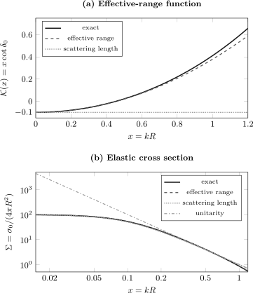
The tuned well has $a=10R$ and $r_e=0.959419R$. The scattering-length approximation keeps the exact $-ik$ unitarity term but replaces $k\cot\delta_0$ by $-1/a$. The effective-range term tracks the exact model much farther toward $kR\sim1$. In the intermediate window $1/a\ll k\ll1/R$, the cross section approaches the $s$-wave unitarity bound.

Three Low-Energy Regimes

The large hierarchy $a/R=10$ separates three momentum regions.

Threshold plateau

When

$$k|a|ll1,$$

or $x\ll0.1$ here,

$$f_0 \simeq -a, \qquad \sigma_0 \simeq 4\pi a^2.$$

The normalized cross section approaches

$$\Sigma(0) = A^2 = 100.$$

Unitary window

If the scale separation is large enough to allow

$$\frac1{|a|} \ll k \ll \frac1R,$$

then $-ik$ dominates over both $-1/a$ and range corrections. The amplitude becomes

$$f_0(k) \simeq \frac{i}{k},$$

and the cross section approaches

$$\sigma_0 \simeq \frac{4\pi}{k^2}.$$

This is the $s$-wave unitarity limit. It is large and nonperturbative even though the collision energy is low.

Range-sensitive regime

When

$$kR \sim 1,$$

the collision resolves the interaction range. The effective range, shape parameter, and eventually higher partial waves matter. Agreement of a low-order formula at one such momentum is not a general universality guarantee.

Numerical Comparison

The exact and approximate normalized cross sections are:

$x=kR$	Exact $\Sigma$	Scattering length	Relative error	Effective range	Relative error
$0.02$	$96.5096$	$96.1538$	$-0.369\%$	$96.5096$	$-9.4\times10^{-6}\%$
$0.10$	$52.4576$	$50.0000$	$-4.68\%$	$52.4560$	$-0.00305\%$
$0.20$	$21.4949$	$20.0000$	$-6.95\%$	$21.4913$	$-0.0170\%$
$0.40$	$6.23036$	$5.88235$	$-5.59\%$	$6.22896$	$-0.0224\%$
$0.60$	$2.73309$	$2.70270$	$-1.11\%$	$2.73759$	$+0.165\%$
$1.00$	$0.855021$	$0.990099$	$+15.8\%$	$0.873989$	$+2.22\%$

Two points deserve emphasis.

First, $kR=0.1$ is small, but the scattering-length result already has a several-percent error. Near the threshold plateau, the relative size of the effective-range term is set by

$$\frac12a r_e k^2,$$

which is enhanced by the large ratio $a/R$.

Second, the excellent effective-range agreement through $x\simeq0.6$ is a property of this benchmark, not a theorem that every short-range potential behaves equally well. The omitted shape term is $O(k^4R^3)$, and its coefficient is model dependent.

Shallow-Bound-State Pole

For a bound state, analytically continue to

$$k=i\kappa, \qquad \kappa>0.$$

The scattering-length amplitude has a pole at

$$\kappa_{\mathrm{univ}} = \frac1a, \qquad \kappa_{\mathrm{univ}}R = 0.1.$$

Its universal binding energy is

$$\frac{E_b^{\mathrm{univ}}}{E_R} = (\kappa R)^2 = 0.01.$$

Including the effective range gives the pole equation

$$-\frac1a - \frac12r_e\kappa^2 + \kappa = 0.$$

The two algebraic roots are

$$\kappa_{\pm} = \frac{1\pm\sqrt{1-2r_e/a}} {r_e}.$$

The shallow root is

$$\kappa_-R = 0.105321201747655.$$

The second root,

$$\kappa_+R = 1.97927473420977,$$

lies beyond the low-energy domain. It must not be promoted to a physical prediction of the truncated expansion.

For the exact square well, write

$$\zeta = \kappa R, \qquad b = \sqrt{g^2-\zeta^2}.$$

Matching the decaying exterior solution gives

$$b\cot b = -\zeta.$$

The shallow exact solution is

$$\zeta_{\mathrm{exact}} = 0.105317031281676,$$

so

$$\frac{E_b^{\mathrm{exact}}}{E_R} = 0.0110916770779855.$$

The scattering-length energy is low by $9.84\%$. The effective-range energy,

$$\frac{E_b^{\mathrm{ERE}}}{E_R} = 0.0110925555375702,$$

differs from the exact result by only $0.00792\%$.

This pole comparison is independent of the positive-energy cross-section table. It tests the analytic continuation of the same low-energy parameters.

What Universality Does and Does Not Say

At leading order, every short-range elastic interaction with the same real scattering length has

$$f_0(k) = -\frac{a}{1+ika}$$

up to range corrections. The microscopic potential may be a square well, a smooth well, a multichannel interaction reduced to one open channel, or a regulated contact theory.

Universality does not say that:

• the wavefunction inside the interaction region is universal;
• the effective range is fixed by the scattering length;
• higher partial waves are always absent;
• inelastic channels can be represented by a real $a$;
• a large positive and large negative $a$ have the same pole interpretation;
• two-body universality determines all three-body observables.

For $a>0$ with $a\gg R$, the pole at $k\simeq i/a$ is a shallow bound state. For $a<0$, the corresponding near-threshold pole lies at $k\simeq-i/|a|$ on the unphysical sheet and is usually called a virtual state. Their leading cross sections depend on $a^2$, but their analytic structures differ.

Error Budget

For the scattering-length amplitude, the first omitted term in $K(k)$ is $r_e k^2/2$. A useful local diagnostic is

$$\epsilon_r(k) = \frac{|r_e|k^2/2} {\max(1/|a|,k)}.$$

This compares the omitted real term with the real or imaginary scale already retained in the denominator. It is a diagnostic rather than a rigorous bound.

For the effective-range approximation, the next term has the form

$$P k^4,$$

where $P$ is a shape parameter with dimensions of length cubed. Natural short-range power counting suggests $P=O(R^3)$ unless a further tuning or long-range tail changes the scale.

A trustworthy numerical test should therefore vary $kR$, compare the extracted $k\cot\delta_0$ rather than only the cross section, and verify that the radial integration domain and matching radius are converged. Phase Shift Extraction gives that workflow.

Identical-Particle Factors

The formulas above use distinguishable-particle normalization:

$$\sigma_0 = 4\pi|f_0|^2.$$

For identical spinless bosons in a pure $s$ wave, symmetrization doubles the amplitude while the final-state phase space must not be counted twice. The result is

$$\sigma_0^{\mathrm{boson}} = 8\pi|f_0|^2.$$

For identical spin-polarized fermions, the spatial state must be antisymmetric and the $s$ wave is forbidden. The leading channel is then usually $p$ wave. Identical-Particle Scattering owns the complete symmetry conventions.

Cross-Checks

1. Dimensions. Both $a$ and $r_e$ have dimensions of length, while $k\cot\delta_0$ has dimensions of inverse length.
2. Threshold. The exact formula gives $\mathcal K(0)=-R/a=-0.1$ and $\Sigma(0)=100$.
3. Unitarity. Every real approximation to $K(k)$ inserted into $[K(k)-ik]^{-1}$ satisfies the elastic single-channel unitarity form.
4. Pole consistency. The same $a$ and $r_e$ describe the positive-energy amplitude and the shallow bound-state continuation.
5. Range counting. The universal and effective-range curves separate only when the collision begins to resolve $R$ or when the large value of $a$ amplifies the nominally small $k^2$ term.
6. Exact benchmark. The physical ERE pole agrees with the exact square-well pole, while the deep algebraic root lies outside the expansion domain.

Common Mistakes

• Replacing $f_0$ by $-a$ when $k|a|$ is not small.
• Calling the scattering-length formula perturbative in $ka$ even though it resums $ika$ exactly.
• Assuming $kR\ll1$ alone guarantees that effective-range corrections are negligible when $|a|/R$ is large.
• Dropping the $-ik$ term and thereby violating the correct elastic unitarity denominator.
• Treating every positive scattering length as evidence for an accurately universal shallow bound state.
• Interpreting the deep root of a truncated effective-range equation as a reliable state.
• Inferring bound versus virtual character from a cross section that depends only on $a^2$.
• Using the distinguishable-particle factor $4\pi$ for identical bosons without checking conventions.
• Applying short-range universality to an unscreened Coulomb interaction.
• Extending the two-body result to three-body physics without the additional parameters required there.

Cross-Links

• Worked Problems and Model Calculations
• Low-Energy Scattering
• Scattering Length
• Effective-Range Expansion
• Partial-Wave Cross Sections
• Unitarity
• Bound States and Scattering Poles
• Identical-Particle Scattering
• Square-Well Scattering
• Hard-Sphere Scattering
• Phase Shift Extraction
• Validity of the Born Approximation

References

• H. A. Bethe, “Theory of the Effective Range in Nuclear Scattering,” Physical Review 76, 38–50 (1949), doi:10.1103/PhysRev.76.38.
• J. M. Blatt and J. D. Jackson, “On the Interpretation of Neutron–Proton Scattering Data by the Schwinger Variational Method,” Physical Review 76, 18–37 (1949), doi:10.1103/PhysRev.76.18.
• J. R. Taylor, Scattering Theory: The Quantum Theory of Nonrelativistic Collisions, Dover, 2006.
• R. G. Newton, Scattering Theory of Waves and Particles, 2nd ed., Dover, 2002.
• L. D. Landau and E. M. Lifshitz, Quantum Mechanics: Non-Relativistic Theory, 3rd ed., Pergamon, 1977.
• E. Braaten and H.-W. Hammer, “Universality in Few-Body Systems with Large Scattering Length,” Physics Reports 428, 259–390 (2006), arXiv:cond-mat/0410417.
• C. Chin, R. Grimm, P. Julienne, and E. Tiesinga, “Feshbach Resonances in Ultracold Gases,” Reviews of Modern Physics 82, 1225–1286 (2010), doi:10.1103/RevModPhys.82.1225.

Exercises

1. Derive the exact effective-range function

Starting from $\tan(x+\delta_0)=T(x)$, derive

$$x\cot\delta_0 = x \frac{1+T(x)\tan x} {T(x)-\tan x}.$$

Solution

Use

$$\tan(x+\delta_0) = \frac{\tan x+\tan\delta_0} {1-\tan x\tan\delta_0} = T.$$

Solving for $\tan\delta_0$ gives

$$\tan\delta_0 = \frac{T-\tan x} {1+T\tan x}.$$

Taking the reciprocal and multiplying by $x$ gives

$$x\cot\delta_0 = x \frac{1+T\tan x} {T-\tan x}.$$

2. Locate the unitary window

For $a=10R$, identify the momentum inequalities required for the universal amplitude to approach $i/k$. Why is the window only parametrically clean rather than broad in this benchmark?

Solution

The scattering-length term is negligible compared with $k$ when

$$k\gg\frac1a = \frac{0.1}{R}.$$

Range corrections remain small when

$$k\ll\frac1R.$$

Thus the desired window is

$$0.1 \ll kR \ll 1.$$

The hierarchy spans only one decade because $a/R=10$. A much larger scattering length would create a broader region in which $1/a$ and $1/R$ are well separated.

3. Explain the enhanced range correction

At $kR=0.1$, estimate the ratio of the effective-range term to $1/a$ and compare it with the cross-section error of the scattering-length approximation.

Solution

The ratio is

$$\frac{r_e k^2/2}{1/a} = \frac12a r_e k^2.$$

Using $a=10R$, $r_e=0.959419R$, and $kR=0.1$ gives

$$\begin{aligned} \frac12a r_e k^2 &= \frac12(10)(0.959419) \,(0.1)^2 \\ &\simeq 0.04797. \end{aligned}$$

The real denominator is shifted by about $4.8\%$, and the exact cross-section comparison shows a $4.68\%$ error. The close numerical agreement is specific to this point, but the scale estimate correctly predicts a several-percent effect.

4. Classify the two effective-range roots

The effective-range pole equation has roots $\kappa_-R=0.105321$ and $\kappa_+R=1.97927$. Explain why only the first is controlled.

Solution

The effective-range expansion is a low-momentum expansion requiring $|k|R\ll1$. The shallow root satisfies

$$\kappa_-R \simeq 0.105,$$

so it lies inside the intended domain and agrees with the exact pole. The second root has $\kappa_+R\simeq1.98$, beyond the range scale. It is an algebraic feature of the truncated quadratic denominator, not a controlled prediction of a second bound state.

5. Change the sign of the scattering length

Keep $|a|=10R$ but take $a<0$ in the scattering-length amplitude. Show that the leading cross section is unchanged and classify the pole.

Solution

The cross section is

$$\sigma_0 = \frac{4\pi a^2} {1+k^2a^2},$$

so it depends only on $a^2$ and is unchanged under $a\to-a$.

The amplitude denominator vanishes at

$$k = \frac{i}{a}.$$

For $a=-|a|$, this is

$$k = -\frac{i}{|a|}.$$

The pole is not a normalizable bound state on the positive imaginary axis. It is the universal near-threshold virtual-state pole on the unphysical sheet.

6. Apply identical-boson counting

For identical spinless bosons with only $s$-wave scattering, derive the factor of two relative to the distinguishable-particle total cross section.

Solution

The symmetrized amplitude is

$$f_{\mathrm B}(\theta) = f(\theta) + f(\pi-\theta).$$

For an isotropic $s$ wave, both terms equal $f_0$, so the amplitude is $2f_0$. Identical final states must not be counted twice, giving

$$\sigma_0^{\mathrm{boson}} = \frac12 \int d\Omega\, |2f_0|^2 = 8\pi|f_0|^2.$$

This is twice the distinguishable result $4\pi|f_0|^2$.