Validity of the Born Approximation

The Born approximation is not valid merely because a potential is called weak or an incident particle is called fast. Its reliability depends on the potential, the collision energy, the angular or partial-wave region, the observable, and the required accuracy.

For nonrelativistic elastic scattering,

$$H=H_0+V, \qquad E=\frac{\hbar^2k^2}{2\mu},$$

the exact outgoing state obeys

$$\lvert\psi_{\mathbf k}^{(+)}\rangle = \lvert\mathbf k\rangle + G_0^{(+)}(E)V \lvert\psi_{\mathbf k}^{(+)}\rangle.$$

The first Born approximation replaces the exact state acted on by $V$ with the incident state:

$$\lvert\psi_{\mathbf k}^{(+)}\rangle \longrightarrow \lvert\mathbf k\rangle.$$

The central validity question is therefore:

Is the distortion generated by $G_0^{(+)}V$ small in the interaction region and for the observable being calculated?

Born Series is the canonical home for the Neumann expansion, its second term, and operator convergence. First Born Approximation derives the leading Fourier-transform formula and examples. This page turns those formal statements into practical tests and failure diagnostics.

State the Claim Precisely

A useful validity statement has at least four qualifiers:

1. Energy range: a method may work at $kR=10$ and fail at $kR=0.1$.
2. Angular or channel range: forward scattering may probe a long coherent path that other angles do not.
3. Observable: a total cross section can be accurate while a diffraction minimum is misplaced.
4. Tolerance: ten-percent accuracy and one-percent accuracy require different evidence.

Thus the statement

$$\text{“Born is valid”}$$

should be replaced by something like:

$$\begin{gathered} \text{“For }2\le kR\le5 \\ \text{and }20^\circ\le\theta\le150^\circ, \\ \text{the first Born differential cross section} \\ \text{agrees with a converged} \\ \text{partial-wave result to within }5\%\text{.”} \end{gathered}$$

No single dimensionless inequality is necessary and sufficient for every potential. The criteria below have different logical status:

Test	What it supplies	Main limitation
interaction-region norm bound	sufficient control in a specified norm	often very conservative
range-and-strength estimate	rapid analytic screening	suppresses geometry and cancellations
high-energy phase estimate	coherent-distortion test	assumes a smooth, localized interaction
partial-wave phases	channel-resolved diagnostic	requires more than the leading Born result for confirmation
second-order or numerical comparison	observable-specific evidence	costs an additional calculation

Range, Strength, and Energy Scales

Suppose a short-range potential has a characteristic range $R$ and a representative magnitude $V_0$. Introduce

$$\kappa=kR$$

and

$$g = \frac{2\mu\lvert V_0\rvert R^2}{\hbar^2}.$$

The first parameter compares the range with the wavelength. The second compares the potential with the kinetic localization scale

$$E_R = \frac{\hbar^2}{2\mu R^2}, \qquad g=\frac{\lvert V_0\rvert}{E_R}.$$

The pointwise energy ratio is

$$\epsilon_E = \frac{\lvert V_0\rvert}{E} = \frac{g}{\kappa^2}.$$

These ratios answer different questions. At low energy, the spatial scale $R$ and the integrated strength of the potential matter. At high energy, the wave accumulates a phase while crossing the interaction region. Consequently, $\lvert V_0\rvert/E\ll1$ by itself can be too weak a test.

A useful scale summary for a smooth finite-range potential is:

Regime	Leading diagnostic	Interpretation
$kR\lesssim1$	$g\ll1$	weak distortion across the full region
$kR\gg1$	$g/(kR)\ll1$	small accumulated phase

Factors of order unity depend on the shape of $V$, the definition of $R$, and the norm or trajectory being tested. These are scaling criteria, not universal sharp boundaries.

Weak-Potential Criterion from the Integral Equation

In coordinate space, define

$$K^{(+)}(E) = G_0^{(+)}(E)V.$$

For the three-dimensional free Hamiltonian,

$$G_0^{(+)} (\mathbf r,\mathbf r';E) = - \frac{\mu}{2\pi\hbar^2} \frac{ e^{ik\lvert\mathbf r-\mathbf r'\rvert} }{ \lvert\mathbf r-\mathbf r'\rvert }.$$

The first correction to a unit-amplitude incident plane wave is

$$\begin{aligned} \delta\psi^{(1)}(\mathbf r) ={}& - \frac{\mu}{2\pi\hbar^2} \int d^3r'\, \frac{ V(\mathbf r') e^{i\mathbf k\cdot\mathbf r'} }{ \lvert\mathbf r-\mathbf r'\rvert } \\ &\times e^{ik\lvert\mathbf r-\mathbf r'\rvert}. \end{aligned}$$

If $D$ is the region in which $V$ is appreciable, a direct diagnostic is

$$\eta_1(k) = \sup_{\mathbf r\in D} \left| \delta\psi^{(1)}(\mathbf r) \right|.$$

For an incident plane wave of unit magnitude, $\eta_1\ll1$ says that the first generated distortion is small where the next interaction would occur. It is much more informative than inspecting $V_0$ alone because it retains energy, geometry, oscillatory cancellation, and the actual incoming state.

Taking absolute values before integration gives the conservative bound

$$\epsilon_{\mathrm{abs}} = \frac{\mu}{2\pi\hbar^2} \sup_{\mathbf r\in D} \int_D d^3r'\, \frac{ \lvert V(\mathbf r')\rvert }{ \lvert\mathbf r-\mathbf r'\rvert }.$$

On bounded functions restricted to $D$,

$$\lVert K^{(+)}\rVert_\infty \le \epsilon_{\mathrm{abs}}.$$

Therefore

$$\epsilon_{\mathrm{abs}}\lt1$$

is a sufficient Neumann-series condition in that restricted norm. It is not necessary: the absolute-value estimate discards all oscillatory cancellation and is usually much stricter than the actual error.

For a potential of magnitude $V_0$ supported in a region of size $R$,

$$\epsilon_{\mathrm{abs}} \sim \frac{\mu\lvert V_0\rvert R^2}{\hbar^2} \sim g,$$

up to a geometry-dependent factor. This explains the weak-coupling scale $g\ll1$.

What a norm bound does not prove

Plane waves are not normalizable vectors in the ordinary Hilbert-space norm, and real-energy resolvents require weighted spaces or a restriction to the interaction region. A quoted operator norm is meaningful only after the function space and domain have been stated.

Moreover, failure of a sufficient bound does not prove failure of the approximation. It only removes that particular guarantee. Oscillation at large $k$ can make the true correction small even when $\epsilon_{\mathrm{abs}}$ is not.

High-Energy Regime

When $kR\gg1$, phases vary rapidly inside a smooth short-range potential. A useful estimate follows from the phase accumulated along an approximately straight trajectory with impact parameter $b$:

$$\chi(b) = - \frac{\mu}{\hbar^2k} \int_{-\infty}^{\infty}dz\, V\left( \sqrt{b^2+z^2} \right).$$

For a region of longitudinal size $R$,

$$\lvert\chi(b)\rvert \sim \frac{\mu\lvert V_0\rvert R}{\hbar^2k} \sim \frac{g}{kR}.$$

The first Born approximation linearizes the interaction-induced phase. A practical high-energy condition is therefore

$$\max_{b\ \mathrm{relevant}} \lvert\chi(b)\rvert \ll1.$$

Equivalently, at the level of scales,

$$\frac{g}{\kappa}\ll1.$$

The relation

$$\frac{g}{\kappa} = \left( \frac{\lvert V_0\rvert}{E} \right) (kR)$$

shows why $\lvert V_0\rvert/E\ll1$ alone is incomplete. A small local energy ratio can accumulate over many wavelengths.

High energy often helps because rapid oscillations suppress repeated propagation through a localized, smooth potential. It does not automatically repair:

• an impenetrable hard core or singular potential;
• an unscreened long-range tail;
• a narrow shape resonance at the chosen energy;
• a channel threshold or strongly coupled inelastic channel;
• a forward observable dominated by a very long coherence length.

The straight-line phase is a diagnostic, not a derivation of every Born amplitude. When $\chi$ is not small but trajectories are still approximately straight, an eikonal resummation may be more appropriate than first Born truncation.

Partial-Wave Test

For a real central potential, the exact elastic amplitude is

$$f(\theta) = \frac{1}{k} \sum_{\ell=0}^{\infty} (2\ell+1) e^{i\delta_\ell} \sin\delta_\ell P_\ell(\cos\theta).$$

The first Born phase shift is

$$\delta_\ell^{(1)}(k) = - \frac{2\mu k}{\hbar^2} \int_0^\infty dr\, r^2V(r)j_\ell^2(kr).$$

Born linearization requires the phase shifts in the contributing channels to be small:

$$\lvert\delta_\ell\rvert\ll1.$$

For a range $R$, the channels most directly sampling the interaction usually satisfy

$$\ell\lesssim kR.$$

This gives a channel-resolved test:

1. compute $\delta_\ell^{(1)}$ for all relevant $\ell$;
2. identify which channels dominate the observable;
3. compare with a second-order estimate or numerically integrated phase shifts;
4. verify convergence as the partial-wave cutoff increases.

Small $\delta_\ell^{(1)}$ is encouraging, but not a proof. Accidental cancellation can make the first-order integral small while a higher-order term remains important.

The exact elastic partial-wave coefficient obeys

$$\left| \frac{ e^{i\delta_\ell}\sin\delta_\ell }{k} \right| \le \frac{1}{k}.$$

A Born prediction approaching or exceeding this scale signals loss of perturbative control. The converse is not guaranteed: staying below a unitarity bound is necessary but not sufficient for accuracy.

Unitarity Must Be Tested Order by Order

For a real potential, the first Born amplitude is real:

$$\operatorname{Im}f^{(1)}(0)=0.$$

Yet its differential cross section is nonzero:

$$\frac{d\sigma^{(2)}}{d\Omega} = \left| f^{(1)}(\theta) \right|^2.$$

This does not by itself invalidate first-order perturbation theory. The optical theorem compares quantities at the same order. Its first nontrivial perturbative statement is

$$\operatorname{Im}f^{(2)}(0) = \frac{k}{4\pi} \int d\Omega\, \left| f^{(1)}(\theta) \right|^2.$$

Thus a useful unitarity test includes the second Born imaginary part. Demanding the exact optical theorem from $f^{(1)}$ alone mixes perturbative orders. Unitarity owns the general order-by-order constraint, Optical Theorem develops the forward relation, and Born Series evaluates its Born terms.

Failure Near Bound States and Resonances

The exact transition operator satisfies

$$T^{(+)} = V + VG_0^{(+)}T^{(+)}.$$

Whenever the indicated inverses exist, the equivalent exact identities are

$$\begin{aligned} T^{(+)} &= V \left( I-G_0^{(+)}V \right)^{-1}, \\ T^{(+)} &= \left( I-VG_0^{(+)} \right)^{-1}V. \end{aligned}$$

A pole appears when an eigenvalue of the iterated kernel approaches unity. Then the inverse contains a small denominator and repeated interactions are enhanced:

$$\left( I-G_0^{(+)}V \right)^{-1} \longrightarrow \text{large}.$$

This mechanism can overwhelm a pointwise weak-potential estimate. Near a bound state, virtual state, or resonance:

• successive Born terms need not decrease;
• observables can vary sharply under a small change of energy or coupling;
• the scattering length can greatly exceed the potential range;
• phase shifts can pass through order-unity values.

The appropriate repair is to solve the relevant channel nonperturbatively, resum the enhanced denominator, or choose a distorted reference Hamiltonian that already contains the pole-producing physics. See Bound States and Scattering Poles for the analytic structure.

Low-Energy s-Wave Warning

For a short-range potential, the low-energy $s$-wave amplitude is

$$f_0(k) = \frac{1}{ k\cot\delta_0(k)-ik }.$$

Using the effective-range expansion,

$$k\cot\delta_0(k) = - \frac{1}{a_s} + \frac{1}{2}r_e k^2 + O(k^4),$$

gives

$$f_0(k) \approx \frac{1}{ -1/a_s+r_e k^2/2-ik }.$$

At threshold,

$$f_0(0)=-a_s.$$

The first Born scattering length is

$$a_s^{(1)} = \frac{\mu}{2\pi\hbar^2} \int d^3r\,V(\mathbf r),$$

or, for a central potential,

$$a_s^{(1)} = \frac{2\mu}{\hbar^2} \int_0^\infty dr\, r^2V(r).$$

This estimate fails dramatically when a state approaches threshold. The attractive spherical square well makes the point with no numerical ambiguity:

$$V(r) = \begin{cases} -V_0, & r\lt R,\\ 0, & r\gt R, \end{cases} \qquad V_0\gt0.$$

Define

$$x = \frac{R\sqrt{2\mu V_0}}{\hbar}.$$

The exact result, derived at Scattering Length, is

$$\frac{a_s}{R} = 1-\frac{\tan x}{x}.$$

First Born theory gives

$$\frac{a_s^{(1)}}{R} = - \frac{x^2}{3}.$$

For $x\ll1$,

$$\frac{a_s}{R} = - \frac{x^2}{3} - \frac{2x^4}{15} + O(x^6),$$

so the Born term is the correct leading weak-coupling limit. At

$$x=\frac{\pi}{2},$$

the first $s$-wave bound state reaches threshold and the exact scattering length diverges. The Born expression has no pole and cannot anticipate the nonperturbative enhancement.

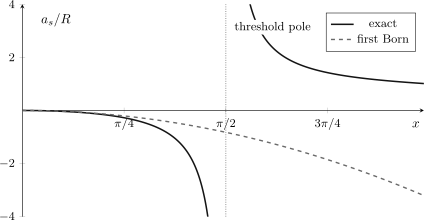
The exact square-well scattering length $a_s/R=1-\tan x/x$ agrees with $a_s^{(1)}/R=-x^2/3$ only at weak coupling. At $x=\pi/2$, a zero-energy state produces a pole that no finite Born truncation can reproduce.

Square-Well Scattering derives the same threshold formula from the exact finite-energy phase shift, verifies its $O(k^2R^2)$ approach to zero energy, and shows a higher-partial-wave shape resonance that is likewise invisible to a naive weak-coupling test.

The warning is especially important because low energy does not mean weak interaction. When

$$\lvert a_s\rvert\gg R,$$

threshold observables are controlled by the nearby pole rather than by a small volume integral of the potential. Low-Energy Scattering owns the universal threshold regime.

Long-Range and Singular Potentials

The ordinary Born construction above assumes that free plane waves are appropriate asymptotic states and that the interaction-region integrals are controlled. Long-range tails can violate both assumptions.

For the unscreened Coulomb potential,

$$V(r)=\frac{\alpha}{r},$$

the absolute interaction-region criterion grows without bound as the region is enlarged. The exact scattering state also contains a logarithmic long-range phase, so the asymptotic form is not simply a plane wave plus an outgoing spherical wave.

The Fourier transform of $1/r$ nevertheless gives a first Born magnitude equal to the Rutherford magnitude. That special agreement does not establish ordinary Born convergence: it misses the full Coulomb phase structure and leaves the forward singularity. Coulomb Scattering gives the canonical treatment.

Possible repairs include:

• introduce physical screening and test the screening-radius limit;
• use Coulomb-distorted incoming and outgoing states;
• split $V=V_{\mathrm{long}}+V_{\mathrm{short}}$ and perturb only the residual short-range interaction.

Hard cores, contact interactions, and potentials singular at the origin raise a different issue. Higher Born integrals may be ultraviolet divergent or cutoff dependent. The remedy is not to assign a small number to an undefined integral; it is to regularize, match or renormalize the interaction, and establish power counting for the regulated problem.

Yukawa Potential in the Born Approximation is a useful intermediate case: its $e^{-\mu r}/r$ core is singular but locally integrable, its screening makes the large-distance transform finite, and an attractive coupling still defeats first order when the first $s$-wave bound state reaches threshold.

Numerical Tests

Analytic scale estimates should be followed by observable-level checks whenever quantitative accuracy matters.

Compare successive terms without dividing by a zero

For

$$f = f^{(1)} + f^{(2)} + \cdots,$$

the ratio

$$\left| \frac{f^{(2)}}{f^{(1)}} \right|$$

is useful only where $f^{(1)}$ is not close to a diffraction zero. Near a zero, report an absolute error or compare cross sections integrated over a finite angular bin:

$$\Delta_\Omega = \frac{ \left| \sigma_\Omega^{(1+2)} - \sigma_\Omega^{(1)} \right| }{ \max\left( \sigma_\Omega^{(1+2)}, \sigma_{\mathrm{scale}} \right) }.$$

The reference scale $\sigma_{\mathrm{scale}}$ prevents a meaningless blow-up when both predictions are negligible.

Sweep an artificial coupling

Replace

$$V\longrightarrow\lambda V$$

and compute the target observable for several small values of $\lambda$. A first Born amplitude should satisfy

$$f(\lambda) = \lambda f^{(1)} + O(\lambda^2),$$

while a cross section away from an amplitude zero should begin as

$$\sigma(\lambda) = \lambda^2\sigma^{(2)} + O(\lambda^3).$$

Curvature, unstable fitted coefficients, or a nearby singular dependence on $\lambda$ exposes enhanced higher orders. The sweep must include enough small couplings to distinguish genuine asymptotic scaling from an accidental fit.

Evaluate the integral-equation residual

Let

$$\phi(\mathbf r) = e^{i\mathbf k\cdot\mathbf r}$$

and form the first-iterated state

$$\psi_1 = \phi+K^{(+)}\phi.$$

Its residual in the exact Lippmann–Schwinger equation is

$$\begin{aligned} \mathcal R_1 &= \psi_1-\phi-K^{(+)}\psi_1 \\ &= - \left( K^{(+)} \right)^2\phi. \end{aligned}$$

Compute a norm of $\mathcal R_1$ on the interaction region and compare it with the norm of $\psi_1$. This directly probes the next omitted state correction. A small residual is evidence only in the chosen norm; it should emphasize the region and channels relevant to the observable.

Benchmark an independent formulation

For a central potential, integrate the radial Schrödinger equation, extract $\delta_\ell$, and reconstruct the amplitude. For a general potential, solve a discretized Lippmann–Schwinger equation. Then verify:

• stability under radial-box or momentum-cutoff enlargement;
• convergence with grid resolution and partial-wave cutoff;
• independence from the finite $i\eta$ regulator after extrapolation;
• agreement of flux and optical-theorem checks;
• convergence over the entire reported energy and angular domain.

Agreement between two calculations is strongest when their numerical errors and analytic assumptions are genuinely independent.

Born Approximation Numerical Test implements this program for a repulsive Gaussian: it sweeps coupling and momentum, resolves radial and partial-wave errors below the Born discrepancy, and compares the error with the largest contributing phase shift.

Practical Decision Procedure

Before reporting a first Born prediction:

1. Classify the interaction. Is it finite range, screened, long range, singular, or coupled-channel?
2. Define scales. State $R$, $V_0$, $kR$, and $g=2\mu\lvert V_0\rvert R^2/\hbar^2$.
3. Check the right regime. Use $g\ll1$ as a conservative low-energy scale and $g/(kR)\ll1$ as a high-energy phase scale when their assumptions apply.
4. Look for poles and thresholds. Inspect scattering lengths, phase shifts, channel openings, and sensitivity to energy or coupling.
5. Test contributing channels. Estimate or compute the relevant partial-wave phases.
6. Calculate one piece of omitted physics. Use a second Born term, a residual, or an independent numerical solution.
7. Validate the observable. Compare amplitudes, phases, or binned cross sections over the stated domain.
8. Report the evidence. Give the diagnostic values and the achieved tolerance, not only the phrase “weak potential.”

When these checks fail, the result is not automatically useless. It may identify the correct qualitative momentum-transfer dependence or provide the first term of an asymptotic expansion. The claim must be narrowed accordingly.

Common Mistakes

• Treating $\lvert V_0\rvert/E\ll1$ as a universal high-energy theorem.
• Applying a sufficient norm bound as though its failure proved the approximation wrong.
• Checking only the total cross section while reporting precise angular minima.
• Dividing by $f^{(1)}$ at a Born zero and interpreting the resulting large ratio literally.
• Demanding the exact optical theorem from the real first Born amplitude alone.
• Ignoring a large scattering length because the potential is shallow pointwise.
• Using free asymptotic states for an unscreened Coulomb tail.
• Trusting apparent numerical agreement before cutoff, grid, and regulator convergence.
• Assuming that a smooth first Born curve can reproduce a nearby pole.

Exercises

Compare the three scale ratios

For a finite-range potential with $kR=20$ and

$$\frac{\lvert V_0\rvert}{E}=10^{-2},$$

find $g$ and $g/(kR)$. Does the pointwise energy ratio alone establish a strongly controlled Born approximation?

Solution

Because

$$\frac{\lvert V_0\rvert}{E} = \frac{g}{(kR)^2},$$

one finds

$$g = 10^{-2}(20)^2 = 4.$$

The accumulated-phase scale is

$$\frac{g}{kR} = \frac{4}{20} = 0.2.$$

The local energy ratio is small, but the coherent phase estimate is only moderately small. Whether $0.2$ is adequate depends on the potential shape, observable, and target tolerance; an explicit next-order or numerical check is needed.

Expand the square-well scattering length

Starting from

$$\frac{a_s}{R} = 1-\frac{\tan x}{x},$$

derive the first two nonzero weak-coupling terms and identify the first Born result.

Solution

The tangent expansion is

$$\tan x = x + \frac{x^3}{3} + \frac{2x^5}{15} + O(x^7).$$

Therefore

$$\begin{aligned} \frac{a_s}{R} &= 1- \left( 1+\frac{x^2}{3} +\frac{2x^4}{15} +O(x^6) \right) \\ &= - \frac{x^2}{3} - \frac{2x^4}{15} + O(x^6). \end{aligned}$$

The term $-x^2/3$ is $a_s^{(1)}/R$. The next correction is negative and of relative order $x^2$ away from the threshold pole.

Reconcile first Born theory with the optical theorem

Why does

$$\operatorname{Im}f^{(1)}(0)=0$$

not contradict the nonzero cross section

$$\int d\Omega\, \lvert f^{(1)}\rvert^2?$$

Solution

The amplitude $f^{(1)}$ is first order in the coupling, while $\lvert f^{(1)}\rvert^2$ is second order. The imaginary forward amplitude required at the same order comes from $f^{(2)}$. Perturbative unitarity reads

$$\operatorname{Im}f^{(2)}(0) = \frac{k}{4\pi} \int d\Omega\, \lvert f^{(1)}(\theta)\rvert^2.$$

Comparing the exact optical theorem with only $f^{(1)}$ mixes first- and second-order quantities.

Derive the first-iteration residual

Let the exact equation be

$$\psi=\phi+K\psi$$

and define $\psi_1=\phi+K\phi$. Show that its residual is $-K^2\phi$.

Solution

Insert $\psi_1$ into the equation residual:

$$\begin{aligned} \mathcal R_1 &= \psi_1-\phi-K\psi_1 \\ &= \left( \phi+K\phi \right) -\phi -K \left( \phi+K\phi \right) \\ &= -K^2\phi. \end{aligned}$$

The residual is precisely the next omitted state correction with a minus sign. Its size in an interaction-region norm is therefore a direct truncation diagnostic.

Diagnose the Coulomb coincidence

The first Born transform of $V(r)=\alpha/r$ reproduces the Rutherford differential cross section. Give two reasons this does not prove that unscreened Coulomb scattering is an ordinary, well-controlled short-range Born problem.

Solution

First, the Coulomb tail changes the asymptotic states by adding logarithmic long-range phases, so free plane waves are not the correct reference states at arbitrarily large distance. Second, the forward amplitude remains singular and the absolute interaction-region estimates do not converge as the region is enlarged. Agreement of the magnitude is a special feature of the Coulomb problem, not evidence that the full phase structure or Born series is controlled.

References

• M. Born, “Quantenmechanik der Stoßvorgänge,” Zeitschrift für Physik 38, 803–827 (1926), doi:10.1007/BF01397184.
• J. R. Taylor, Scattering Theory: The Quantum Theory of Nonrelativistic Collisions, Dover, 2006, Chapters 9–11.
• R. G. Newton, Scattering Theory of Waves and Particles, 2nd ed., Springer, 1982, Chapters 11 and 12.
• C. J. Joachain, Quantum Collision Theory, 3rd ed., North-Holland, 1983, Chapters 6 and 7.
• M. L. Goldberger and K. M. Watson, Collision Theory, Wiley, 1964, Chapters 3 and 4.
• T. Jacobson, “Features of the Born Approximation,” University of Maryland PHYS 623 lecture note, PDF.
• S. Weinberg, “Quasiparticles and the Born Series,” Physical Review 131, 440–460 (1963), doi:10.1103/PhysRev.131.440.