Born Series

The Born series is the stationary scattering expansion generated by repeated interactions with a potential. Its first term describes one interaction, its second term describes two interactions separated by free propagation, and higher terms continue the same pattern.

For the transition operator,

$$\begin{aligned} T^{(+)}(E) ={}& V \\ &+ VG_0^{(+)}(E)V \\ &+ VG_0^{(+)}(E) V \\ &\qquad\times G_0^{(+)}(E)V + \cdots. \end{aligned}$$

This is a Neumann series for an exact integral equation. Writing the terms is always possible formally; claiming that the infinite series converges, or that a short truncation is accurate, requires additional evidence.

This page is the canonical home for Born iteration, order counting, the second Born term, convergence, and repeated-scattering failure modes. Lippmann–Schwinger Equation owns the exact state equation, T-Matrix owns the exact transition operator and its normalization, First Born Approximation owns leading-order applications, and Validity of the Born Approximation translates formal control into range, energy, channel, and numerical diagnostics.

The name has no direct connection to the Born probability rule or the Born–Oppenheimer approximation.

Introduce a Coupling Parameter

Write

$$H(\lambda) = H_0+\lambda V,$$

where $\lambda$ counts powers of the interaction. It may be a physical coupling or a bookkeeping parameter. If it is only bookkeeping, set $\lambda=1$ after the expansion and its validity have been analyzed.

For elastic relative motion,

$$E_{\mathbf k} = \frac{\hbar^2k^2}{2\mu},$$

and the outgoing free resolvent is

$$G_0^{(+)}(E) = \frac{1}{E-H_0+i0}.$$

Use delta-normalized wave-number states,

$$\begin{aligned} \langle\mathbf r\vert\mathbf k\rangle &= (2\pi)^{-3/2} e^{i\mathbf k\cdot\mathbf r}, \\ \langle\mathbf k'\vert\mathbf k\rangle &= \delta^{(3)} (\mathbf k'-\mathbf k). \end{aligned}$$

With these conventions, the on-shell amplitude and transition operator are related by

$$\begin{aligned} f(\mathbf k',\mathbf k) ={}& -\frac{4\pi^2\mu}{\hbar^2} \\ &\times \langle\mathbf k'\vert T^{(+)}(E_{\mathbf k}) \vert\mathbf k\rangle. \end{aligned}$$

Every Born-order formula below inherits this normalization.

Iterating the State Equation

The outgoing Lippmann–Schwinger equation is

$$\lvert\psi_\lambda^{(+)}\rangle = \lvert\phi\rangle + \lambda G_0^{(+)}V \lvert\psi_\lambda^{(+)}\rangle.$$

Define the fixed-energy scattering kernel

$$K^{(+)} \equiv G_0^{(+)}(E)V.$$

Then

$$\left( I-\lambda K^{(+)} \right) \lvert\psi_\lambda^{(+)}\rangle = \lvert\phi\rangle.$$

Formally expanding the inverse gives

$$\begin{aligned} \lvert\psi_\lambda^{(+)}\rangle ={}& \sum_{n=0}^{\infty} \lambda^n \left(K^{(+)}\right)^n \lvert\phi\rangle \\ ={}& \lvert\phi\rangle + \lambda G_0^{(+)}V \lvert\phi\rangle \\ &+ \lambda^2G_0^{(+)}V G_0^{(+)}V \lvert\phi\rangle + \cdots. \end{aligned}$$

The zeroth-order state is the incident free state. The order-$\lambda^n$ correction has interacted $n$ times and contains $n$ factors of $V$.

In coordinate space, one iteration is

$$\begin{aligned} \psi^{(1)}(\mathbf r) ={}& \int d^3r_1\, G_0^{(+)} (\mathbf r,\mathbf r_1;E) \\ &\qquad\times V(\mathbf r_1) \phi(\mathbf r_1). \end{aligned}$$

The next iteration integrates over two possible interaction points:

$$\begin{aligned} \psi^{(2)}(\mathbf r) ={}& \int d^3r_2\,d^3r_1\, G_0^{(+)} (\mathbf r,\mathbf r_2;E) \\ &\times V(\mathbf r_2) G_0^{(+)} (\mathbf r_2,\mathbf r_1;E) \\ &\times V(\mathbf r_1) \phi(\mathbf r_1). \end{aligned}$$

Each Green function carries the wave freely from one interaction point to the next with the same outgoing boundary prescription.

Iterating the Transition Operator

For $H(\lambda)=H_0+\lambda V$, the transition operator obeys

$$T_\lambda^{(+)} = \lambda V + \lambda V G_0^{(+)} T_\lambda^{(+)}.$$

Write

$$T_\lambda^{(+)} = \sum_{n=1}^{\infty} \lambda^nT^{(n)}.$$

Matching powers of $\lambda$ gives

$$\begin{aligned} T^{(1)} &= V, \\ T^{(2)} &= VG_0^{(+)}V, \\ T^{(3)} &= VG_0^{(+)}VG_0^{(+)}V, \end{aligned}$$

and, in general,

$$\begin{aligned} T^{(n)} &= V \left( G_0^{(+)}V \right)^{n-1} \\ &= \left( VG_0^{(+)} \right)^{n-1} V. \end{aligned}$$

The amplitude has the corresponding expansion

$$f = \sum_{n=1}^{\infty} \lambda^n f^{(n)},$$

where

$$\begin{aligned} f^{(n)} (\mathbf k',\mathbf k) ={}& -\frac{4\pi^2\mu}{\hbar^2} \\ &\times \langle\mathbf k'\vert T^{(n)} \vert\mathbf k\rangle. \end{aligned}$$

The state series begins at order $\lambda^0$, while the transition amplitude begins at order $\lambda^1$. Confusing those two starting orders is a common source of off-by-one terminology.

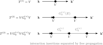
The first three transition-operator terms. Read each process from the incoming state $\mathbf k$ on the left to the outgoing state $\mathbf k'$ on the right. In the operator product acting on a ket, the rightmost factor acts first. These are fixed-energy potential-scattering diagrams, not automatically QFT Feynman diagrams.

First Born Term

The first term is

$$T^{(1)}=V.$$

For a local potential, define

$$\begin{aligned} \widetilde V(\mathbf q) &= \int d^3r\, e^{-i\mathbf q\cdot\mathbf r} V(\mathbf r), \\ \mathbf q &= \mathbf k'-\mathbf k. \end{aligned}$$

Then

$$\langle\mathbf k'\vert V \vert\mathbf k\rangle = \frac{ \widetilde V(\mathbf q) }{ (2\pi)^3 },$$

so

$$f^{(1)}(\mathbf q) = -\frac{\mu}{2\pi\hbar^2} \widetilde V(\mathbf q).$$

This is the first Born approximation when all higher terms are omitted. It is one interaction in the amplitude, not one power in the cross section: $|f^{(1)}|^2$ is already order $\lambda^2$.

Gaussian, Yukawa, and central-potential transforms are worked out in First Born Approximation.

Second Born Term

The second term is the first one that contains an intermediate propagation:

$$T^{(2)} = V G_0^{(+)}(E)V.$$

Insert a complete set of free momentum states:

$$\begin{aligned} &\langle\mathbf k'\vert T^{(2)} \vert\mathbf k\rangle \\ &\quad= \int d^3p\, \frac{ \langle\mathbf k'\vert V\vert\mathbf p\rangle }{ E_{\mathbf k}-E_{\mathbf p}+i0 } \\ &\qquad\quad\times \langle\mathbf p\vert V\vert\mathbf k\rangle. \end{aligned}$$

The external momenta are on shell,

$$|\mathbf k'|=|\mathbf k|,$$

but the intermediate momentum $\mathbf p$ ranges over all values. It is generally off shell.

The distribution identity

$$\frac{1}{x+i0} = \operatorname{PV}\frac{1}{x} - i\pi\delta(x)$$

splits the second term into a dispersive principal-value integral and an absorptive on-shell contribution:

$$\begin{aligned} &\langle\mathbf k'\vert T^{(2)} \vert\mathbf k\rangle \\ ={}& \operatorname{PV} \int d^3p\, \frac{ V_{\mathbf k'\mathbf p} V_{\mathbf p\mathbf k} }{ E_{\mathbf k}-E_{\mathbf p} } \\ &- i\pi \int d^3p\, \delta \left( E_{\mathbf k}-E_{\mathbf p} \right) \\ &\qquad\times V_{\mathbf k'\mathbf p} V_{\mathbf p\mathbf k}, \end{aligned}$$

where

$$V_{\mathbf a\mathbf b} \equiv \langle\mathbf a\vert V\vert\mathbf b\rangle.$$

For a Hermitian potential in the forward direction,

$$\begin{aligned} \operatorname{Im} \langle\mathbf k\vert T^{(2)} \vert\mathbf k\rangle ={}& -\pi \int d^3p\, \delta \left( E_{\mathbf k}-E_{\mathbf p} \right) \\ &\qquad\times \left| V_{\mathbf p\mathbf k} \right|^2 \le0. \end{aligned}$$

The amplitude normalization has an additional minus sign, so $\operatorname{Im}f^{(2)}(0)\ge0$.

In the unit-incident-amplitude coordinate convention, the same term is

$$\begin{aligned} f^{(2)} (\mathbf k',\mathbf k) ={}& -\frac{\mu}{2\pi\hbar^2} \int d^3r\,d^3r'\, e^{-i\mathbf k'\cdot\mathbf r} \\ &\times V(\mathbf r) G_0^{(+)} (\mathbf r,\mathbf r';E) \\ &\times V(\mathbf r') e^{i\mathbf k\cdot\mathbf r'}. \end{aligned}$$

This form makes the physical order explicit: interact at $\mathbf r'$, propagate freely to $\mathbf r$, then interact again before reaching the far field.

Perturbative Unitarity

For one-channel elastic scattering,

$$\operatorname{Im}f(0) = \frac{k}{4\pi} \int d\Omega\, |f(\Omega)|^2.$$

Insert

$$f = \lambda f^{(1)} + \lambda^2f^{(2)} + O(\lambda^3).$$

For a Hermitian potential, the forward first Born matrix element is real. Matching order $\lambda^2$ gives

$$\operatorname{Im}f^{(2)}(0) = \frac{k}{4\pi} \int d\Omega\, \left| f^{(1)}(\Omega) \right|^2.$$

The on-shell delta term in $G_0^{(+)}$ supplies exactly this imaginary part. Therefore the vanishing of $\operatorname{Im}f^{(1)}(0)$ does not contradict the nonzero leading cross section. Comparing $\operatorname{Im}f^{(1)}$ with $|f^{(1)}|^2$ mixes perturbative orders.

Optical Theorem owns the exact relation. Common Failure Modes develops the order-consistency diagnostic.

When the Neumann Series Converges

The algebraic identity

$$\left( I-\lambda K^{(+)} \right)^{-1} = \sum_{n=0}^{\infty} \lambda^n \left(K^{(+)}\right)^n$$

is valid in operator norm if the series converges in the function space being used. A simple sufficient condition is

$$|\lambda|\, \left\| K^{(+)} \right\| \lt1.$$

If the state series is truncated after order $N$,

$$\lvert\psi_{\lambda,N}^{(+)}\rangle = \sum_{n=0}^{N} \lambda^n \left(K^{(+)}\right)^n \lvert\phi\rangle,$$

then the exact remainder is

$$\begin{aligned} \lvert R_N\rangle ={}& \left( \lambda K^{(+)} \right)^{N+1} \\ &\times \left( I-\lambda K^{(+)} \right)^{-1} \lvert\phi\rangle. \end{aligned}$$

Under the sufficient norm condition,

$$\begin{aligned} \lVert R_N\rVert \le{}& \frac{ \left( |\lambda| \lVert K^{(+)}\rVert \right)^{N+1} }{ 1- |\lambda| \lVert K^{(+)}\rVert } \\ &\times \lVert\phi\rVert. \end{aligned}$$

This is a genuine bound only after the space, norm, and boundedness assumptions have been stated.

An ideal incident plane wave does not have a finite global $L^2$ norm. The bound must therefore be applied to a wave packet, a weighted or local norm, or a source such as $V\lvert\phi\rangle$ restricted to the interaction region.

At a continuum energy, $G_0^{(+)}$ is not a bounded operator on unweighted $L^2(\mathbb R^3)$. Scattering convergence is instead formulated with localized interaction regions, weighted spaces, or other mappings for which $G_0^{(+)}V$ is controlled. In a finite discretization, the corresponding matrix norm or spectral radius can be inspected, but the result may depend on box size, regulator, and basis cutoff.

The norm condition is sufficient, not necessary for a useful low-order approximation. Cancellations can make selected matrix elements accurate even when a global norm is pessimistic. Conversely, a small first correction at one angle can be caused by a zero and need not imply convergence elsewhere.

Poles Set the Dangerous Scale

The exact state is

$$\lvert\psi_\lambda^{(+)}\rangle = \left( I-\lambda K^{(+)} \right)^{-1} \lvert\phi\rangle.$$

Under the usual analytic and compactness hypotheses, singularities in complex $\lambda$ occur when $I-\lambda K^{(+)}$ ceases to be invertible. Those singularities limit the radius of the power series about $\lambda=0$. At fixed physical coupling, a nearby bound-state or resonance pole in energy likewise amplifies repeated scattering.

An inverse may exist even when its geometric expansion does not converge. In one scalar eigenchannel with

$$K^{(+)}\to\kappa,$$

the exact factor is $(1-\lambda\kappa)^{-1}$, but the Born sum

$$1+\lambda\kappa + (\lambda\kappa)^2+\cdots$$

converges only for $|\lambda\kappa|\lt1$. For example, $\lambda\kappa=-2$ gives a finite exact inverse $1/3$ and a divergent geometric series.

This is why “the exact integral equation has a solution” and “the Born series converges” are different claims.

Practical Diagnostics

No single ratio diagnoses every scattering problem. Useful checks include:

• compute $f^{(2)}$ and compare it with $f^{(1)}$ over the full angular and energy range of interest;
• avoid the ratio $f^{(2)}/f^{(1)}$ near symmetry or diffraction zeros of the leading term;
• scale $V\to\lambda V$ numerically and verify the predicted powers of $\lambda$;
• compare with a direct solution of the Lippmann–Schwinger equation;
• compare with partial-wave phase shifts for a central potential;
• test the optical theorem order by order;
• vary the regulator, domain size, momentum cutoff, and quadrature;
• inspect whether a bound state, virtual state, threshold, or resonance lies nearby.

The dedicated Small Parameters and Error Estimates page distinguishes rigorous bounds from such error indicators.

Failure Modes

Strong or resonant scattering

If repeated action of $G_0^{(+)}V$ is not small, successive terms need not decrease. Near a pole, many orders can be equally important and a finite truncation can miss the dominant physics.

Thresholds and shallow states

At low energy, the free resolvent is enhanced and the $s$-wave scattering length can become much larger than the potential range. A potential that looks weak pointwise can be nonperturbative because it nearly supports a bound state.

Long-range interactions

For an unscreened Coulomb potential, free asymptotic states and the ordinary short-range Born series are not the correct starting point. A distorted-wave expansion should incorporate the long-range interaction into the reference Hamiltonian.

Singular interactions and cutoffs

Higher Born integrals can be ultraviolet sensitive for contact or singular potentials. A cutoff-dependent term is not a prediction until the interaction has been regularized and its parameters matched or renormalized.

Several channels

An intermediate state may run through every coupled channel, including closed channels. Near an opening threshold, channel momenta and branch points can invalidate smooth single-channel power counting.

Improving the Starting Point

The split $H=H_0+V$ is not unique. If a known part of the interaction is strong or long ranged, write

$$H=H_{\mathrm{ref}}+W$$

and expand in the residual interaction $W$ using

$$G_{\mathrm{ref}}^{(+)}(E) = \frac{1}{ E-H_{\mathrm{ref}}+i0 }.$$

This produces a distorted-wave Born series. A better reference Hamiltonian can move essential physics into the zeroth-order states and make the residual iteration smaller.

Other options include:

• solving the integral equation directly;
• using partial waves and enforcing elastic unitarity channel by channel;
• resumming a separable or otherwise structured interaction;
• using Padé or related rational approximants with independent pole and convergence checks;
• replacing the potential description by a low-energy effective theory with matched couplings.

Resummation is not automatically more accurate. It is trustworthy only when its analytic assumptions and calibration are controlled.

Diagrammatic Intuition and the QFT Warning

The repeated-interaction picture resembles a diagram expansion:

• each $V$ is an interaction insertion;
• each $G_0^{(+)}(E)$ is fixed-energy free propagation;
• each intermediate momentum is integrated;
• the external momenta are put on shell when an observable amplitude is extracted.

This resemblance does not identify Born order with QFT loop order. A second Born term contains an intermediate-momentum integral, but in field-theory matching it often represents an iterated, two-particle-reducible contribution already generated by the nonrelativistic equation. A QFT loop can also contain irreducible short-distance physics, relativistic energy integration, antiparticles, and renormalization.

The safe correspondence is:

1. match the irreducible low-energy interaction kernel or potential to QFT;
2. iterate that kernel with the nonrelativistic Green function when the power counting requires it;
3. subtract or avoid contributions already generated by iteration.

Otherwise the same physics can be counted twice. QFT Bridge: Born Approximation and Tree Level develops the leading-order comparison, while Bridge to QFT Scattering explains the broader normalization and LSZ changes.

The Born series is also distinct from the time-dependent Dyson series. Dyson ordering integrates interaction times; the Born series iterates a stationary fixed-energy resolvent. They can encode related perturbative physics, but their terms are organized in different representations.

Common Mistakes

• Treating a formal iteration as proof of convergence.
• Calling $V$ small without specifying a dimensionless operator, matrix-element, or partial-wave criterion.
• Forgetting that the state series begins at order zero while the amplitude begins at order one.
• Calling $VG_0V$ “one scattering” because it is the first correction to $T=V$.
• Restricting the intermediate momentum in the second Born term to the external energy shell.
• Dropping the $i0$ prescription and losing the imaginary part required by unitarity.
• Testing the optical theorem with terms from different perturbative orders.
• Inferring convergence from a small correction at one accidental zero.
• Applying the free Born series to unscreened Coulomb scattering.
• Ignoring cutoff dependence in singular higher-order integrals.
• Equating a Born iteration with a QFT loop or counting both in a matched calculation.
• Assuming a resummation is accurate merely because it produces a finite answer.

Cross-Links

• Lippmann–Schwinger Equation
• Green Function for Scattering
• T-Matrix
• First Born Approximation
• Optical Theorem
• Partial-Wave Expansion
• Bound States and Scattering Poles
• Coulomb Scattering
• Small Parameters and Error Estimates
• Common Failure Modes
• QFT Bridge: Born Approximation and Tree Level
• Dyson Expansion as Formal Time Evolution

References

1. M. Born, “Quantenmechanik der Stoßvorgänge”, Zeitschrift für Physik 38, 803–827 (1926).
2. B. A. Lippmann and J. Schwinger, “Variational principles for scattering processes. I”, Physical Review 79, 469–480 (1950).
3. M. Gell-Mann and M. L. Goldberger, “The formal theory of scattering”, Physical Review 91, 398–408 (1953).
4. J. R. Taylor, Scattering Theory: The Quantum Theory of Nonrelativistic Collisions, Dover (2006).
5. R. G. Newton, Scattering Theory of Waves and Particles, 2nd ed., Dover (2002).
6. M. L. Goldberger and K. M. Watson, Collision Theory, Dover (2004).
7. C. J. Joachain, Quantum Collision Theory, 3rd ed., North-Holland (1983).
8. M. Reed and B. Simon, Methods of Modern Mathematical Physics, Vol. III: Scattering Theory, Academic Press (1979).

Exercises

Match the state and transition orders

Starting from

$$\lvert\psi_\lambda^{(+)}\rangle = \lvert\phi\rangle + \lambda G_0^{(+)}V \lvert\psi_\lambda^{(+)}\rangle,$$

derive $\psi^{(0)}$, $\psi^{(1)}$, $\psi^{(2)}$, and the corresponding first three transition-operator terms.

Solution

Insert

$$\lvert\psi_\lambda^{(+)}\rangle = \sum_{n=0}^{\infty} \lambda^n \lvert\psi^{(n)}\rangle.$$

Matching powers gives

$$\begin{aligned} \lvert\psi^{(0)}\rangle &= \lvert\phi\rangle, \\ \lvert\psi^{(1)}\rangle &= G_0^{(+)}V \lvert\phi\rangle, \\ \lvert\psi^{(2)}\rangle &= G_0^{(+)}V G_0^{(+)}V \lvert\phi\rangle. \end{aligned}$$

Since

$$T_\lambda^{(+)} \lvert\phi\rangle = \lambda V \lvert\psi_\lambda^{(+)}\rangle,$$

the transition terms are

$$\begin{aligned} T^{(1)} &= V, \\ T^{(2)} &= VG_0^{(+)}V, \\ T^{(3)} &= VG_0^{(+)}VG_0^{(+)}V. \end{aligned}$$

Recover the second-order imaginary part

For Hermitian $V$, use the second Born momentum integral to show that

$$\operatorname{Im} \langle\mathbf k\vert T^{(2)} \vert\mathbf k\rangle \le0.$$

Why does this give a nonnegative $\operatorname{Im}f^{(2)}(0)$ in the convention of this page?

Solution

The imaginary part comes from

$$\frac{1}{ E_{\mathbf k}-E_{\mathbf p}+i0 } \supset -i\pi \delta \left( E_{\mathbf k}-E_{\mathbf p} \right).$$

Hermiticity gives

$$\langle\mathbf k\vert V\vert\mathbf p\rangle \langle\mathbf p\vert V\vert\mathbf k\rangle = \left| \langle\mathbf p\vert V\vert\mathbf k\rangle \right|^2.$$

Therefore

$$\begin{aligned} \operatorname{Im}T_{\mathbf k\mathbf k}^{(2)} ={}& -\pi \int d^3p\, \delta \left( E_{\mathbf k}-E_{\mathbf p} \right) \\ &\times \left| V_{\mathbf p\mathbf k} \right|^2 \le0. \end{aligned}$$

Because

$$f^{(2)} = -\frac{4\pi^2\mu}{\hbar^2} T^{(2)}$$

on shell, the extra negative factor makes $\operatorname{Im}f^{(2)}(0)\ge0$.

Prove the Neumann remainder bound

Let $A=\lambda K^{(+)}$ and assume $\lVert A\rVert\lt1$. Show that truncating

$$(I-A)^{-1} = \sum_{n=0}^{\infty}A^n$$

after $A^N$ produces a remainder bounded by

$$\frac{ \lVert A\rVert^{N+1} }{ 1-\lVert A\rVert }.$$

Solution

The remainder is

$$\begin{aligned} \sum_{n=N+1}^{\infty}A^n &= A^{N+1} \sum_{m=0}^{\infty}A^m \\ &= A^{N+1}(I-A)^{-1}. \end{aligned}$$

Submultiplicativity and the geometric bound give

$$\begin{aligned} \left\| \sum_{n=N+1}^{\infty}A^n \right\| &\le \lVert A\rVert^{N+1} \sum_{m=0}^{\infty} \lVert A\rVert^m \\ &= \frac{ \lVert A\rVert^{N+1} }{ 1-\lVert A\rVert }. \end{aligned}$$

Applying this operator to $\lvert\phi\rangle$ adds a factor $\lVert\phi\rVert$.

Separate invertibility from convergence

In a scalar eigenchannel, take $\lambda\kappa=-2$. Compare the exact inverse $(1-\lambda\kappa)^{-1}$ with the corresponding Born geometric series.

Solution

The inverse exists and equals

$$\frac{1}{1-(-2)} = \frac{1}{3}.$$

The Born series is

$$1-2+4-8+\cdots,$$

whose terms do not approach zero, so it diverges. Existence of the exact inverse therefore does not imply convergence of its expansion about $\lambda=0$ at the chosen coupling.

Identify the double-counting risk

A QFT calculation is matched to a nonrelativistic potential, and that potential is then iterated in the Lippmann–Schwinger equation. Why should a field-theory contribution equal to the same two-particle-reducible iteration not also be added independently to the potential?

Solution

The Lippmann–Schwinger equation already generates

$$VG_0^{(+)}V$$

from two insertions of the matched potential. Adding the identical reducible contribution to the potential kernel and then iterating would count it once in matching and again in the dynamical equation. Matching should isolate the irreducible kernel appropriate to the chosen power counting, while reducible propagation is generated by the nonrelativistic Green function.