Central-Field Approximation

The central-field approximation replaces the coupled motion of many atomic electrons by one-electron motion in an effective spherically symmetric potential. The potential contains the nuclear attraction and an averaged description of the other electrons. Its eigenfunctions provide orbitals, subshells, and a reference configuration; residual interactions then refine or mix that reference.

This page owns the atomic meaning and diagnostics of that reduction. Hartree Method owns the self-excluded atomic direct field and coupled radial iteration. The general variational derivations of Hartree theory and Hartree–Fock theory remain canonical in Many-Body and Quantum Statistical Mechanics. A central field may be motivated by those methods, by a fitted model potential, or by a spherical average of a more elaborate calculation. Those origins are not interchangeable, so the construction must be stated.

The Many-Electron Problem

For $N$ nonrelativistic electrons and a point nucleus of charge $+Ze$, the fixed-nucleus Hamiltonian in Hartree atomic units is

$$H=\sum_{i=1}^{N} \left(-\frac12\nabla_i^2-\frac{Z}{r_i}\right) +\sum_{i<j}\frac{1}{r_{ij}}.$$

The nuclear term is central, but the electron–electron term depends on the angle between $\mathbf r_i$ and $\mathbf r_j$ as well as their radii. It couples electron coordinates and prevents the wavefunction from factorizing into exact independent orbitals.

The central-field strategy chooses a reference Hamiltonian

$$H_0=\sum_{i=1}^{N}h_{\mathrm{cf}}(i),$$

with

$$h_{\mathrm{cf}} =-\frac12\nabla^2+V_{\mathrm{cf}}(r).$$

The difference

$$H_{\mathrm{res}}=H-H_0$$

contains whatever two-electron interaction and one-electron counterterms were not absorbed into $V_{\mathrm{cf}}$. Calling $H_{\mathrm{res}}$ “small” is a hypothesis to test, not a consequence of writing this decomposition.

What Central Means

A local central potential depends only on $r$. Therefore

$$[h_{\mathrm{cf}},L^2]=0, \qquad [h_{\mathrm{cf}},L_z]=0.$$

One-electron orbitals can be written

$$\phi_{n\ell m\sigma}(\mathbf r,s) =\frac{P_{n\ell}(r)}{r} Y_\ell^m(\theta,\phi)\chi_\sigma(s),$$

where $\chi_\sigma$ is a spin function. The radial orbital satisfies

$$\begin{aligned} h_{\ell}^{\mathrm{rad}} &=T_{\ell}^{\mathrm{rad}}+V_{\mathrm{cf}}(r),\\ T_{\ell}^{\mathrm{rad}} &=-\frac12\frac{d^2}{dr^2} +\frac{\ell(\ell+1)}{2r^2},\\ h_{\ell}^{\mathrm{rad}}P_{n\ell}(r) &=\epsilon_{n\ell}P_{n\ell}(r). \end{aligned}$$

Spherical symmetry guarantees the $2\ell+1$ degeneracy in $m$ before external fields or nonspherical interactions are included. Unlike the pure Coulomb problem, a generic central potential does not make different $\ell$ values at the same principal label degenerate. The orbital energy normally depends on both $n$ and $\ell$.

A central field is a model, not a literal force from a frozen cloud

The phrase “each electron feels the average field of the others” is useful but incomplete. In a self-consistent theory, the orbitals create a density, the density creates an effective operator, and that operator changes the orbitals. For fermions, exchange is generally nonlocal; correlation is not captured by a simple average density. A fitted local potential may reproduce selected energies without being the Hartree field of any unique density.

Screening and Effective Charge

Write a local effective potential schematically as

$$V_{\mathrm{cf}}(r) =-\frac{Z}{r}+V_{\mathrm{screen}}(r).$$

The screening term is positive for the direct electrostatic repulsion from other electrons. It weakens the nuclear attraction experienced by an electron, but it is not generally equivalent to replacing $Z$ by one constant.

For a spherical number density $\rho(r)$ of other electrons, normalized to their number, the direct Hartree potential in atomic units is

$$\begin{aligned} V_H(r)=4\pi\biggl[ &\frac{1}{r}\int_0^r \rho(r')r'^2\,dr'\\ &+\int_r^\infty \rho(r')r'\,dr' \biggr]. \end{aligned}$$

Charge inside radius $r$ contributes as if concentrated at the origin; charge outside contributes a spatially constant potential within each spherical shell. The result follows from the spherical average of the Coulomb kernel, not from assuming every electron occupies a sharp shell.

Near and far from the nucleus

At small $r$, the singular nuclear attraction dominates:

$$V_{\mathrm{cf}}(r) \sim-\frac{Z}{r} \qquad(r\to0).$$

Far outside all other electrons, an electron sees the net charge of the nucleus plus the remaining $N-1$ electrons. If the ion has charge $q=Z-N$, then

$$V_{\mathrm{cf}}(r) \sim-\frac{q+1}{r} \qquad(r\to\infty).$$

For a neutral atom, $q=0$, so a distant valence electron sees an asymptotic $-1/r$ tail. For a singly positive ion, the tail is $-2/r$. This asymptotic charge is a stringent diagnostic for model potentials intended to describe Rydberg states or ionization.

When the potential is local, one may define a radius-dependent effective charge by

$$Z_{\mathrm{eff}}(r)=-rV_{\mathrm{cf}}(r).$$

It approaches $Z$ near the nucleus and $q+1$ far away under the ideal limits above. A single tabulated “effective nuclear charge” is therefore an orbital-dependent approximation to a function, not an exact property of the atom.

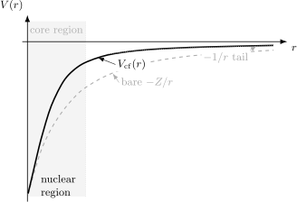
Schematic local potentials for a neutral atom. Near the nucleus, both retain the $-Z/r$ singularity. Through the core region, electron screening weakens the attraction, and the effective valence potential approaches $-1/r$ at large $r$. A real self-consistent or fitted potential need not follow the particular interpolation drawn here.

Penetration and Orbital-Dependent Screening

Orbitals with different $\ell$ sample the core differently. The centrifugal term

$$\frac{\ell(\ell+1)}{2r^2}$$

suppresses low-radius amplitude increasingly as $\ell$ grows. At comparable principal excitation:

• $s$ orbitals penetrate the core most strongly;
• $p$ orbitals generally penetrate less;
• $d$ and $f$ orbitals are often concentrated farther outside the core;
• stronger penetration exposes an electron to a larger effective nuclear charge and usually increases its binding.

This ordering is qualitative, not a universal theorem about every level. Radial nodes, core relaxation, relativistic contraction, near-degeneracy, and configuration mixing can change simple expectations.

Screening is not shielding by rigid shells

Electron density is continuous and orbitals overlap. Inner electrons do not create a perfectly opaque barrier, and outer electrons still contribute to self-consistent fields. Shell language organizes the density and angular momenta; it should not be converted into a classical picture of nested charged surfaces.

Shells, Subshells, and Configurations

The central-field orbitals are labeled $n\ell m\sigma$. Pauli exclusion allows at most one electron per spin-orbital. A spatial subshell of given $n\ell$ therefore has capacity

$$2(2\ell+1).$$

Subshell	$\ell$	Spatial orbitals	Maximum electrons
$s$	$0$	$1$	$2$
$p$	$1$	$3$	$6$
$d$	$2$	$5$	$10$
$f$	$3$	$7$	$14$

An electron configuration records occupation of these subshells, for example $1s^22s^22p^6$. It is a basis-level description of a reference state. An exact many-electron eigenstate can be a superposition of configurations, and open-shell levels require coupling the individual orbital and spin angular momenta into total $L$, $S$, and $J$.

Electron Configurations is the canonical guide to occupation notation, Aufbau reasoning and its limits, closed-shell and valence partitions, and configuration mixing.

Orbital energies are not the many-electron spectrum

The eigenvalue $\epsilon_{n\ell}$ belongs to an effective one-electron equation. The total energy includes interaction double counting and depends on the chosen approximation. Excitation energies are differences of many-electron state energies, not generally differences of frozen central-field orbital eigenvalues. Koopmans-type relations add assumptions such as a single determinant and frozen relaxation; they are not exact identities for measured spectra.

Quantum Defects

A valence or Rydberg electron in a neutral alkali atom sees an asymptotic $-1/r$ potential but departs from a pure Coulomb potential in the core. A Rydberg series is often represented by

$$E_{n\ell j} \simeq E_{\mathrm{ion}} -\frac{hcR_MZ_c^2} {(n-\delta_{\ell j})^2},$$

where $Z_c=q+1$ is the residual core charge, $R_M$ uses the appropriate mass convention, and

$$n^*=n-\delta_{\ell j}$$

is the effective principal quantum number. The quantum defect $\delta_{\ell j}$ summarizes the short-range phase accumulated when the electron penetrates and polarizes the core.

Low-$\ell$ series usually have larger defects because they penetrate more strongly. High-$\ell$ Rydberg states remain mostly outside the core and become nearly hydrogenic. Fine structure can make the defect $j$ dependent.

What a quantum defect is not

A defect is not a missing fraction of an electron, a literal change in $n$, or a universal constant of an element. It can depend on energy, isotope, ionization threshold, channel coupling, and the fitting convention. Near perturbing configurations, a constant-defect model may fail and multichannel quantum-defect methods or explicit configuration mixing may be required.

The NIST atomic-spectroscopy compendium gives the evaluated spectroscopic convention for term series and quantum defects.

Rydberg Atoms Basics uses $n^*$ to organize the large-orbit, polarizability, lifetime, and interaction scalings that follow from this effective one-electron picture.

How Central Fields Are Constructed

Different constructions answer different questions.

Construction	Effective operator	What it includes	Characteristic limitation
screened Coulomb model	chosen local $V(r)$	qualitative penetration and shell ordering	fitted parameters may not transfer between observables
Hartree	local direct field	self-consistent density response	inadmissible raw product for identical electrons; self-interaction and no exchange
Hartree–Fock	direct plus nonlocal exchange	determinant antisymmetry and exchange	no correlation beyond one determinant
central-field Hartree–Fock	spherical average of open shells	atomic subshell structure with exchange	nonspherical and configuration effects are averaged
local density-functional model	local effective potential	exchange-correlation approximation through the density	orbital energies and functional errors require interpretation
model potential fitted to data	local or nonlocal effective operator	selected observed energies or phase shifts	may lack a unique variational or microscopic meaning

The Hartree Approximation and Hartree–Fock Approximation pages own the full restricted-variation derivations. Hartree–Fock for Atoms develops the spherical closed-shell reduction, open-shell averages, and radial exchange multipoles. A local central potential cannot exactly reproduce a general nonlocal exchange operator for every orbital simultaneously.

Self-consistent-field loop

A typical atomic calculation proceeds as follows:

1. choose trial radial orbitals or a trial density;
2. construct direct and, if used, exchange operators;
3. solve the one-electron equations;
4. rebuild the density from the occupied orbitals;
5. mix old and new fields if needed for numerical stability;
6. iterate until stated energy, density, and residual criteria converge;
7. test alternative initial states, occupations, and symmetries;
8. evaluate observables and corrections with a method consistent with the converged reference.

Numerical convergence to a fixed point does not prove that the state is the lowest stable solution or that the approximation is accurate. Stability, basis convergence, and observable-level benchmarks are separate checks.

Residual Interactions and Configuration Mixing

Once $H_0$ is chosen, the residual operator can be treated perturbatively or by diagonalization in a configuration basis. Schematically,

$$|\Psi_{\Gamma}\rangle =\sum_I c_I^{(\Gamma)}|\Phi_I\rangle,$$

where $|\Phi_I\rangle$ are antisymmetrized configuration-state functions with the required total symmetry. The coefficients encode mixing that a single configuration cannot represent.

Residual electrostatic interactions split terms, spin–orbit interactions mix or split angular-momentum couplings, and near-degenerate configurations can invalidate low-order perturbation theory. The central field remains useful as a basis generator even when it is not itself an accurate final-state description.

When the Approximation Works

The central-field picture is often effective when:

• the spherical part of the nuclear and electronic potential dominates;
• one configuration has a large amplitude in the states of interest;
• residual interactions are small compared with relevant configuration separations;
• a closed-shell core is compact and weakly polarizable for the observable considered;
• valence motion is well represented by an effective one-electron potential;
• orbital and quantum-defect labels vary smoothly along a series.

It can still be useful qualitatively outside this regime, but labels should then be presented as dominant components rather than exact identities.

Failure Modes

The approximation becomes unreliable or incomplete when:

• configurations are nearly degenerate or strongly mixed;
• open shells produce important nonspherical multipole fields;
• exchange or correlation changes level ordering or transition amplitudes;
• core polarization and core excitation are comparable to valence separations;
• autoionizing or continuum channels couple strongly to bound configurations;
• high precision requires Breit, QED, recoil, or nuclear corrections;
• strong external fields destroy the spherical symmetry used to define $\ell$ and $m$;
• a local potential is asked to reproduce observables governed by nonlocal exchange or energy-dependent channels.

No single scalar error estimate covers all observables. Energies, oscillator strengths, hyperfine constants, polarizabilities, and scattering phases probe different parts of the approximate state.

Observable-Level Validation

A central-field calculation should be judged against the observables it is meant to predict. Agreement of a total energy alone is not enough: two approximations can have similar energies but substantially different radial orbitals, tails, and transition matrix elements.

Internal checks

Before comparing with experiment, verify that the numerical problem has actually been solved:

• occupied orbitals are normalized and mutually orthogonal when the method requires it;
• the self-consistent residual and changes in energy and density meet stated tolerances;
• results are stable under enlargement of the radial box, basis, grid, and angular-momentum cutoff;
• the density integrates to the intended electron number;
• the potential has the correct nuclear and large-$r$ limits;
• alternative starting occupations do not reveal a lower or unstable solution with the required symmetry.

For a local potential, substituting a computed radial orbital back into the radial equation gives a direct residual test. A small self-consistent-field energy change can coexist with a poor orbital residual if the stopping criterion is badly chosen.

External checks

The most informative benchmarks depend on the intended use:

Intended use	Useful diagnostics
shell ordering and spectroscopy	ionization energies, term intervals, level crossings, and quantum defects
radial structure	expectation values, isotope shifts, hyperfine constants, and electron-scattering form factors
electric-dipole transitions	line strengths, branching ratios, lifetimes, and length-versus-velocity-form consistency
response properties	static and dynamic polarizabilities, Stark shifts, and oscillator-strength sum rules
continuum processes	scattering phase shifts, threshold behavior, photoionization cross sections, and resonance positions

Length and velocity forms of an oscillator strength agree for exact states used with a consistent Hamiltonian. Their disagreement in a truncated calculation is therefore a useful warning, although agreement is not by itself proof of accuracy. Likewise, satisfying a sum rule can expose missing strength but does not guarantee that each individual line is correct.

Validate the tail separately

Weakly bound states, Rydberg series, polarizabilities, tunneling rates, and threshold scattering are especially sensitive to the long-range potential. A model fitted to compact low-lying orbitals may have the wrong asymptotic charge or omit the polarization tail

$$V_{mathrm{pol}}(r)sim -\frac{\alpha_c}{2r^4},$$

where $\alpha_c$ is the static dipole polarizability of the residual core in atomic units. This term is weaker than the Coulomb tail but can matter once the leading Coulomb behavior is fixed. It must not be inserted twice if core polarization is already represented by the underlying many-body method or fitted potential.

Practical Workflow

For a new atom or ionic sequence, a defensible central-field analysis usually follows this order:

1. State the Hamiltonian and conventions. Specify finite or infinite nuclear mass, nuclear charge model, relativistic level, and atomic-unit conventions.
2. Choose the reference configuration. Record occupations and the total symmetry or spherical averaging prescription, especially for open shells.
3. Choose the construction. Distinguish a fitted screened potential, Hartree, Hartree–Fock, density-functional, or other effective operator.
4. Enforce the correct limits. Check the $-Z/r$ nuclear singularity for a point nucleus and the asymptotic charge appropriate to the residual ion.
5. Converge the one-electron problem. Report basis or grid tests as well as self-consistent-field thresholds.
6. Identify the residual physics. Estimate configuration mixing, core polarization, relativistic terms, recoil, and radiative corrections at the precision being claimed.
7. Benchmark the target observable. Use data or a higher-level calculation that probes the same radial and angular structure.
8. Attach uncertainty to the observable, not just the orbitals. The error budget should follow the quantity reported.

The resulting orbitals are often best regarded as a coordinate system for organizing a many-electron calculation. Their usefulness does not require treating each orbital energy or configuration label as directly observable.

Common Mistakes

• Replacing screening by one universal $Z_{\mathrm{eff}}$. Penetration makes screening depend on radius and orbital; a single fitted charge is usually observable- and state-dependent.
• Treating shells as rigid charged spheres. Electronic densities overlap and respond to occupation, so the field is not produced by impermeable screening layers.
• Equating orbital energies with all excitation energies. Relaxation, exchange, correlation, and configuration mixing distinguish energy differences from independent-particle orbital gaps.
• Filling orbitals without antisymmetrizing. A list of occupations is not yet a valid fermionic many-electron state; Slater determinants or symmetry-adapted combinations are required.
• Assuming every central field is self-consistent. Empirical and model potentials can be central without being generated by the density of their own orbitals.
• Assuming convergence proves accuracy. Iteration can converge tightly to an unstable, metastable, or systematically biased approximation.
• Using one quantum defect everywhere. Defects can depend on energy, $j$, isotope, threshold, and channel coupling.
• Expecting a local potential to reproduce nonlocal exchange exactly. A local surrogate can fit selected quantities, but it does not become the Hartree–Fock exchange operator.
• Reading configuration labels as exact identities. In strongly mixed states, labels name dominant components and must be accompanied by mixing information.

Exercises

1. Asymptotic charge seen by an outer electron

An atom or ion has nuclear charge $Z$ and $N$ electrons. Let $q=Z-N$ be its net charge in units of $e$. Place one electron far outside the other $N-1$ electrons. Show that its leading potential energy is

$$V(r)\sim -\frac{q+1}{r}.$$

What does this become for a neutral atom?

Solution

At distances much larger than the core, only its total charge enters the monopole field. The nucleus contributes $+Z$, while the other $N-1$ electrons contribute $-(N-1)$. The residual core charge is therefore

$$Z-(N-1)=Z-N+1=q+1.$$

The active electron has negative charge, so its potential energy is $-(q+1)/r$. For a neutral atom, $q=0$ and the tail is $-1/r$: far away, the electron sees the singly charged ion left after its removal. Multipole and polarization terms fall faster with $r$.

2. Subshell capacity

Derive the maximum number of electrons in a subshell with orbital angular momentum $\ell$. Evaluate the result for $p$ and $d$ subshells.

Solution

For fixed $\ell$, the magnetic quantum number takes $2\ell+1$ values,

$$m=-\ell,-\ell+1,\ldots,\ell.$$

Each spatial orbital can be combined with two spin states. Pauli exclusion therefore gives

$$g_{\ell}=2(2\ell+1).$$

Thus a $p$ subshell, with $\ell=1$, holds $6$ electrons, while a $d$ subshell, with $\ell=2$, holds $10$. This count does not determine the term structure within a partly filled subshell; residual electrostatic and spin-dependent interactions still split the allowed many-electron states.

3. Penetration from quantum defects

Two Rydberg series converge to the same threshold and share the same mass-corrected Rydberg constant. At $n=12$, suppose an $s$ series has $\delta_s=3.00$ and a $d$ series has $\delta_d=0.02$. Compute their effective principal quantum numbers and the ratio of their binding-energy magnitudes in the constant-defect model.

Solution

The effective principal quantum numbers are

$$\begin{aligned} n_s^*&=12-3.00=9.00,\\ n_d^*&=12-0.02=11.98. \end{aligned}$$

Because $|E-E_{mathrm{ion}}|\propto 1/(n^*)^2$,

$$\frac{|E_s-E_{\mathrm{ion}}|}{|E_d-E_{\mathrm{ion}}|} =\left(\frac{11.98}{9.00}\right)^2 \approx 1.77.$$

The larger $s$-wave defect signals stronger penetration into the core and a substantially larger binding magnitude at the same nominal $n$. The numerical defects are model inputs here; near perturbers, an energy-independent defect may not be adequate.

4. Which degeneracy survives?

Explain why a generic spin-independent central potential keeps the $m$ degeneracy for fixed $n\ell$ but does not preserve the hydrogenic degeneracy between different $\ell$ values at fixed $n$.

Solution

A central Hamiltonian commutes with $L^2$ and $L_z$. Rotational invariance makes all $2\ell+1$ orientations of a given orbital equivalent, so the energy is independent of $m$. Different $\ell$ values, however, obey radial equations with different centrifugal terms,

$$\frac{\ell(\ell+1)}{2r^2},$$

and they penetrate a screened core differently. Rotational symmetry does not connect them. The pure Coulomb problem has an additional conserved Runge–Lenz vector and an enlarged dynamical symmetry, which produces the accidental $\ell$ degeneracy. A generic $V(r)$ lacks that symmetry.

5. Accurate energies, poor oscillator strengths

A one-configuration central-field calculation reproduces several level energies to within one percent, but its electric-dipole oscillator strengths disagree strongly with measured branching ratios. Give at least three plausible reasons and outline a useful response.

Solution

Plausible causes include configuration mixing that changes transition amplitudes more than energies, core polarization, inconsistent treatment of the transition operator, incorrect radial tails, and cancellation between several amplitude contributions. In variational calculations, an energy can also be less sensitive to a small wavefunction error than a matrix element is.

A useful response is to inspect the dominant configuration-state amplitudes, compare length and velocity forms using a consistent Hamiltonian, enlarge the configuration space, add core-polarization or response corrections without double counting, and benchmark lifetimes or several related lines rather than one fitted transition. The appropriate remedy follows the observable-level diagnosis; refitting a scalar screening charge to the energies alone need not improve the amplitudes.

Cross-Links

• Common Atomic Hamiltonians records the central-field reference and residual-interaction subtraction beside other standard atomic baselines.
• Hydrogen as Atomic Prototype identifies which Coulomb features survive screening and which are special to the one-electron problem.
• Alkali Atoms applies a screened one-active-electron model to D lines, quantum defects, hyperfine manifolds, cooling, clocks, and Rydberg states.
• Rydberg Atoms Basics develops high-$n$ scaling and long-range pair interactions from the same core-plus-valence model.
• Atomic Orbitals Revisited explains which parts of an orbital description are state, basis, subspace, or method dependent.
• Electron Configurations owns the subshell-occupation language built on a central-field reference and its relation to mixed eigenstates.
• Periodic Table from Quantum Mechanics uses screened subshell energetics to explain period lengths, ionization trends, and their limits.
• Hartree Method derives the self-consistent spherical direct field, self-excluded asymptotic tail, and atomic SCF checks.
• Hartree–Fock for Atoms adds the nonlocal exchange channel and open-shell atomic prescriptions.
• Atomic Units and Scales supplies the unit system used in the radial and many-electron Hamiltonians above.
• Central Potentials is the canonical home for separation of a one-particle central-potential problem.
• Pauli Exclusion Principle and Slater Determinants develop the fermionic state-space structure behind configurations.
• Mean-Field Theory, Hartree Approximation, and Hartree–Fock Approximation own the general variational and self-consistent-field derivations.
• Two-Body Operators gives the operator language for the Coulomb interaction and its residual part.
• Helium Variational Estimate is a compact example of screening represented by an optimized effective charge.

References

1. D. R. Hartree, “The Wave Mechanics of an Atom with a Non-Coulomb Central Field. Part I. Theory and Methods,” Proceedings of the Cambridge Philosophical Society 24, 89–110 (1928), doi:10.1017/S0305004100011919.
2. V. Fock, “Näherungsmethode zur Lösung des quantenmechanischen Mehrkörperproblems,” Zeitschrift für Physik 61, 126–148 (1930), doi:10.1007/BF01340294.
3. R. D. Cowan, The Theory of Atomic Structure and Spectra (University of California Press, 1981), especially Chapters 3–8.
4. W. R. Johnson, Atomic Structure Theory: Lectures on Atomic Physics (Springer, 2007), doi:10.1007/978-3-540-68013-0.
5. E. U. Condon and G. H. Shortley, The Theory of Atomic Spectra (Cambridge University Press, 1935), Chapters 6–9.
6. B. H. Bransden and C. J. Joachain, Physics of Atoms and Molecules, 2nd ed. (Pearson, 2003), Chapters 6–8.
7. C. J. Foot, Atomic Physics (Oxford University Press, 2005), Chapters 3–5.
8. A. Kramida, Y. Ralchenko, J. Reader, and the NIST ASD Team, NIST Atomic Spectra Database, National Institute of Standards and Technology, doi:10.18434/T4W30F.
9. National Institute of Standards and Technology, Atomic Spectroscopy: Term Series, Quantum Defects, and Spectral-Line Conventions.