Spectroscopy

Spectroscopy is the experimental practice of separating radiation by wavelength or frequency and using the resulting spectrum to identify matter, measure transitions, and test models. It was one of the decisive techniques behind quantum mechanics because atoms and molecules emit and absorb radiation at sharply reproducible frequencies.

This page treats spectroscopy as an instrument family and evidence pipeline. The historical atomic line story lives in Line Spectra, Balmer Formula, and Rydberg Formula. The modern hydrogen calculation lives in Hydrogen Atom and Hydrogen Spectrum.

What a Spectroscope Does

A spectroscope takes radiation from a source, spreads it according to wavelength or frequency, and records intensity as a function of that variable. Historically, prisms and diffraction gratings were central dispersive elements. Modern spectrometers may use gratings, interferometers, cavities, lasers, heterodyne detection, frequency combs, or Fourier-transform methods.

The essential output is a spectrum:

intensity versus wavelength, frequency, wavenumber, or photon energy

The independent variable matters. Optical spectroscopy often reports wavelength $\lambda$, frequency $\nu$, angular frequency $\omega$, photon energy $E$, or wavenumber $\tilde\nu$. In vacuum,

$$\nu = \frac{c}{\lambda}, \qquad \omega=2\pi\nu, \qquad E=h\nu, \qquad \tilde\nu=\frac{1}{\lambda}.$$

Historical tables often use wavelength or wavenumber. Modern quantum mechanics often interprets the same data as energy differences.

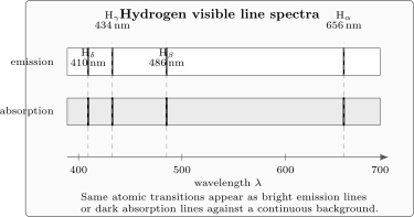
Hydrogen line spectra made the spectral problem concrete: reproducible line positions required an account of discrete transition frequencies, not arbitrary classical radiation from continuously variable orbits.

Emission Spectra

An emission spectrum is produced when a source radiates at characteristic frequencies. A low-pressure gas discharge is the clean historical example: atoms are excited by collisions or fields, then emit photons as they return to lower-energy states.

In modern language, an emitted photon connects an initial state of energy $E_i$ to a lower final state of energy $E_f$:

$$h\nu = E_i-E_f, \qquad E_i>E_f.$$

That compact formula should not be read back into the nineteenth century too quickly. Early spectroscopists saw bright lines before they had energy eigenstates, Hilbert spaces, or transition amplitudes. The experimental regularity came first.

Emission spectra are powerful because line positions are reproducible fingerprints. Sodium’s yellow doublet, hydrogen’s Balmer lines, mercury lines, and many other examples showed that chemical species carry internal frequency scales. Classical electrodynamics alone did not explain why atoms of the same element should emit such stable discrete patterns.

Absorption Spectra

An absorption spectrum is produced when broadband radiation passes through matter and selected frequencies are removed or weakened. In a simple model,

$$I(\nu) = I_0(\nu)\,e^{-\tau(\nu)},$$

where $I_0(\nu)$ is the incident intensity and $\tau(\nu)$ is the optical depth. Absorption lines appear where the medium has allowed transitions that take energy from the radiation field.

The same transition frequency can appear as emission or absorption. In emission, an excited system radiates downward. In absorption, an incoming photon drives an upward transition:

$$h\nu = E_f-E_i, \qquad E_f>E_i.$$

This reciprocity made spectroscopy a chemical and astronomical tool. Laboratory emission lines could be compared with dark solar absorption lines, allowing elements to be identified in remote sources. For quantum mechanics, the key lesson was that the same internal energy differences control both processes.

Spectral Resolution

Spectroscopy is only as good as its ability to distinguish nearby lines. A common figure of merit is resolving power:

$$R = \frac{\lambda}{\Delta\lambda} = \frac{\nu}{\Delta\nu},$$

where $\Delta\lambda$ or $\Delta\nu$ is the smallest separation that can be distinguished under the stated criterion.

Resolution is limited by many effects:

• the optical design of the spectrometer;
• slit width, detector pixel size, and alignment;
• finite observation time;
• Doppler broadening from thermal motion;
• collisions and pressure broadening;
• natural linewidth from finite excited-state lifetime;
• unresolved hyperfine, isotope, or Zeeman structure.

Natural linewidth gives a useful scale. If an excited state has lifetime $\tau$, the line cannot be infinitely sharp; a rough frequency width is

$$\Delta\nu_{\mathrm{nat}} \sim \frac{1}{2\pi\tau}.$$

Thermal motion gives another standard scale. For particles of mass $m$ at temperature $T$, Doppler broadening has a fractional size of order

$$\frac{\Delta\nu}{\nu} \sim \sqrt{\frac{k_B T}{mc^2}},$$

up to convention-dependent numerical factors.

The experimental warning is important: a line position, a line width, and a line intensity are different observables. A theory that predicts the frequency but not the strength or width is incomplete as a spectroscopy theory.

Atomic Identification

Spectroscopy became a method of identification because elements have characteristic patterns of lines. A single line can be suggestive, but reliable identification usually needs a pattern:

• multiple lines with consistent wavelength calibration;
• expected relative strengths under the source conditions;
• absence of plausible contaminant lines;
• agreement across emission or absorption contexts;
• awareness of isotope, ionization, pressure, and temperature effects.

The Bunsen–Kirchhoff program made this logic systematic. A clean flame or discharge source, a dispersive spectroscope, and careful comparison of line positions turned spectra into chemical evidence. The discovery of cesium and rubidium by their spectral lines made the point dramatically: spectroscopy could identify matter that ordinary chemical inspection had missed.

Modern databases continue this work with critically evaluated wavelengths, energy levels, and transition probabilities. The experimental context remains essential. A database line list is not automatically an identification; it is a reference against which calibrated, modeled spectra are compared.

Quantum Transitions

In modern quantum mechanics, spectral lines are transitions between states. The frequency is set by an energy difference:

$$\nu_{fi} = \frac{E_f-E_i}{h}.$$

But a frequency condition is not enough. The strength of a transition depends on a matrix element. For an electric-dipole transition, the relevant operator is proportional to the dipole moment $\mathbf d$, and the strength involves quantities of the form

$$\lvert \langle f\rvert \mathbf d\cdot\boldsymbol\epsilon \lvert i\rangle \rvert^2,$$

where $\boldsymbol\epsilon$ is the light polarization. If symmetry forces this matrix element to vanish, the transition is forbidden in that approximation.

This is where spectroscopy connects to the mature formalism:

• energy eigenvalues give line positions;
• matrix elements give transition strengths;
• angular momentum and parity give selection rules;
• perturbation theory gives transition probabilities and rates;
• line shapes reveal lifetimes, motion, collisions, and environments.

For the formal bridge, see First-Order Transition Probability, Fermi’s Golden Rule, Transition Rates in Light–Matter Interaction, Selection Rules, Dipole Transitions, Applications to Atomic Spectra, Selection Rules and Transition Rates, and Wigner–Eckart Theorem.

Modern Spectroscopy Bridge

Modern spectroscopy is much broader than nineteenth-century optical line observation. It includes microwave spectroscopy, infrared spectroscopy, Raman spectroscopy, laser spectroscopy, magnetic resonance, photoelectron spectroscopy, X-ray spectroscopy, neutron spectroscopy, and precision frequency metrology.

The quantum-mechanical theme is shared:

prepare a system, drive or observe a transition, resolve frequencies,
and infer structure from energies, matrix elements, and line shapes.

Laser spectroscopy made this theme extraordinarily precise. Narrow linewidths, tunability, saturated absorption, laser cooling, trapped ions, atomic clocks, and frequency combs turned spectroscopy into a precision test of quantum electrodynamics, fundamental constants, and many-body environments.

At the same time, spectroscopy remains model-dependent. A peak must be assigned to a transition, molecule, isotope, material band, resonance, or background process. The apparatus produces data; quantum theory supplies the state and transition framework that makes the data interpretable.

Common Pitfalls

• Treating every spectral line as if it comes from a literal electron jumping between Bohr orbits.
• Confusing wavelength in air with wavelength in vacuum.
• Reading line intensity as population alone without considering matrix elements, selection rules, detector response, and optical depth.
• Ignoring line broadening when comparing measured spectra to ideal energy differences.
• Treating a database match as proof of identification without checking calibration and contamination.
• Forgetting that continuous spectra also exist; spectroscopy does not imply that every energy spectrum is discrete.

Cross-Links

• Spectroscopy Chapter Overview
• Absorption and Emission
• Infrared Spectroscopy
• Raman Spectroscopy
• Experimental Techniques and Instruments
• Line Spectra
• Balmer Formula
• Rydberg Formula
• Franck–Hertz Experiment
• Bohr Model
• Zeeman Effect Revisited
• Observables Before Operators
• Transition Probabilities
• First-Order Transition Probability
• Resonant Driving
• Fermi’s Golden Rule
• Transition Rates in Light–Matter Interaction
• Selection Rules
• Dipole Transitions
• Applications to Atomic Spectra
• Selection Rules and Transition Rates
• Hydrogen Spectrum
• Atomic Spectra

References

• G. Kirchhoff and R. Bunsen, “Chemical Analysis by Spectrum-Observations,” Philosophical Magazine 20, 89-109, 1860.
• J. J. Balmer, “Notiz ueber die Spectrallinien des Wasserstoffs,” Annalen der Physik und Chemie 25, 80-87, 1885.
• J. R. Rydberg, “Recherches sur la constitution des spectres d’emission des elements chimiques,” Kungliga Svenska Vetenskapsakademiens Handlingar 23, 1-177, 1890.
• G. Herzberg, Atomic Spectra and Atomic Structure, Dover, 1944.
• W. Demtröder, Laser Spectroscopy: Basic Concepts and Instrumentation, 4th ed., Springer, 2008.
• A. Kramida, Yu. Ralchenko, J. Reader, and NIST ASD Team, NIST Atomic Spectra Database, version 5.12, NIST Standard Reference Database 78, DOI: 10.18434/T4W30F.

Exercises

1. A spectral line is measured at vacuum wavelength $656.3\,\mathrm{nm}$. Compute its frequency to two significant figures.

Solution

Use $\nu=c/\lambda$ with $c\approx3.00\times10^8\,\mathrm{m/s}$ and $\lambda=656.3\times10^{-9}\,\mathrm m$:

$$\nu = \frac{3.00\times10^8}{656.3\times10^{-9}} \approx 4.57\times10^{14}\,\mathrm{Hz}.$$

To two significant figures, $\nu\approx4.6\times10^{14}\,\mathrm{Hz}$.

2. A spectrometer has resolving power $R=50{,}000$ near $\lambda=500\,\mathrm{nm}$. Estimate the wavelength separation $\Delta\lambda$ it can resolve.

Solution

Use $R=\lambda/\Delta\lambda$:

$$\Delta\lambda = \frac{\lambda}{R} = \frac{500\,\mathrm{nm}}{50{,}000} = 0.010\,\mathrm{nm}.$$

3. Why is a line position not enough to predict line intensity?

Solution

The line position is mainly set by an energy difference. The intensity also depends on populations, transition matrix elements, selection rules, line broadening, optical depth, detector response, and source geometry. Two transitions can have similar frequencies but very different strengths.

4. Why did absorption spectra help connect laboratory spectroscopy to astronomy?

Solution

Atoms and ions can absorb at the same characteristic transition frequencies at which they emit. Laboratory emission lines could therefore be compared with dark absorption lines in sunlight or starlight. Matching line patterns made it possible to identify elements in remote objects.